The full computation for konbini40426 used a total of roughly 43 years of computer time if run on a single processor core of one of our Linux servers. The main computations were carried out in October and November of 2024 at the University of Waterloo on a network of 10 servers, each with 32 cores. The TSP computation ran when the servers were not otherwise busy with day-to-day projects.
After initial checks of the OSRM distance table, I sent the konbini40426 TSPLIB file to Keld Helsgaun, the creator of the LKH code and all-around tour-finding expert. Sixteen hours later, Keld wrote "LKH+MERGE found a Konbini tour of length 35578434." After another week, Keld found two more tours of this same length. Based on past experience with LKH results on large map instances, we were, at this point, confident that 35578434 must be very close to the shortest-possible value for konbini40426. It took another 8 weeks before we eventually proved that it is not only close, it is in fact the optimum.
In the computation that produced the optimality proof, we followed standard practice and initiated our branch-and-bound search with an upper bound of 1 greater than the best-known tour length, to force the search to reproduce an optimal solution (as a check on the run). But having the strong bound at the start was a great help in the computation.
The initial bound guides the Concorde code in a number of ways. It allows for subproblems to be pruned in the branch-and-bound search, it lets the code eliminate edges that cannot be in any tour better than the initial bound, and it sets the tolerances for switching between faster and slower routines for finding cutting planes.
But for the largest instances we study, such as konbini40426, the greatest help the LKH tour provides is on the human-decision side. For more modest-size instances, such as the 13,571-stop 7-Eleven tour, we can typically just hit the Concorde start button with default settings and wait for the optimal solution. This is not case for the largest instances, where we are pushing the limits of solvability to study potential improvements in the solution process. Here we are making adjustments on-the-fly, switching between the cutting-plane method and branch-and-bound search, experimenting with new cutting-plane routines, testing branching rules, and more. These choices depend heavily on the gap between the lower bound we are computing and the upper bound given by the best-known tour. So go LKH+MERGE.
The key to proving a tour is shortest possible is to construct a linear-programming (LP) relaxation for the TSP instance, that is, an LP model such that every TSP tour is a candidate solution. If the optimal LP value (or, more generally, the value of any dual LP solution) is β, then no tour can have length less than β. That is, β is a lower bound for the TSP, giving us a means to establish a quality guarantee on the length of our tour.
An LP model for the TSP assigns to every point-to-point connection a (possibly fractional) value between 0 and 1. A point-to-point connection joins a pair of stops; it is called a link or an edge. A tour can be represented as an LP solution where every link is assigned either 0 or 1; the links assigned the value 1 correspond to those that are used in the tour. The LP constraints are rules that are satisfied by all tour solutions. A basic rule, called a degree equation, is that for every stop the values of the links meeting the stop must sum to two. An important further rule, called a subtour inequality, is that for any subset of stops S, the values of the links having one end in S and the other end not in S must be at least two.
An LP solution that has all values 0 or 1 and satisfies all degree equations and subtour inequalities is a tour. Great, but an LP solution might have fractional values. This is where the difficult work of the cutting-plane method starts. The process adds more and more rules, increasing the lower bound β and forcing the LP solution to be closer to all 0-1 values.
During October, we slowly built our LP relaxation, using Concorde's implementation of the cutting-plane method to repeatedly improve the LP's quality, that is, to increase the lower bound it produced.
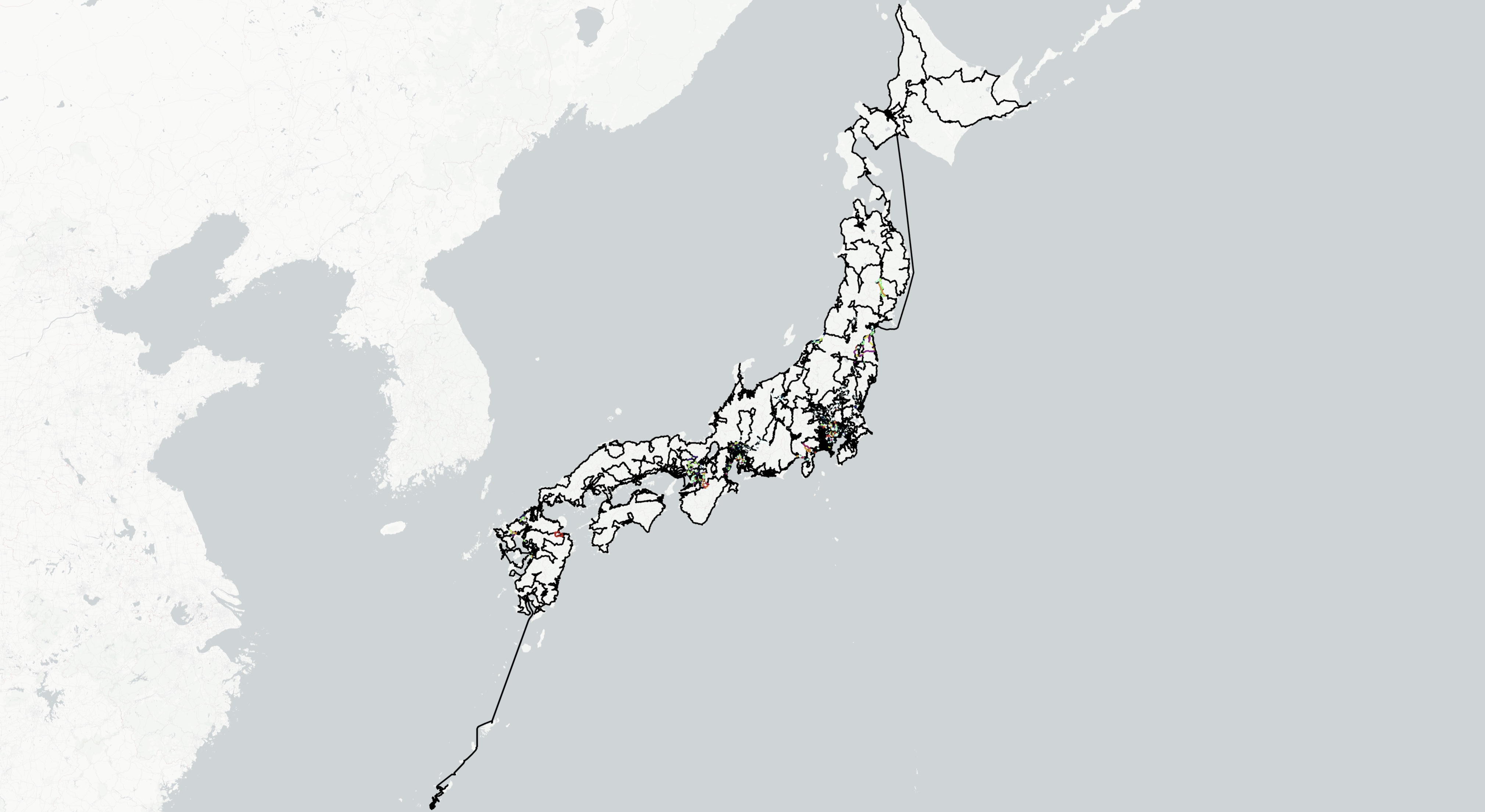
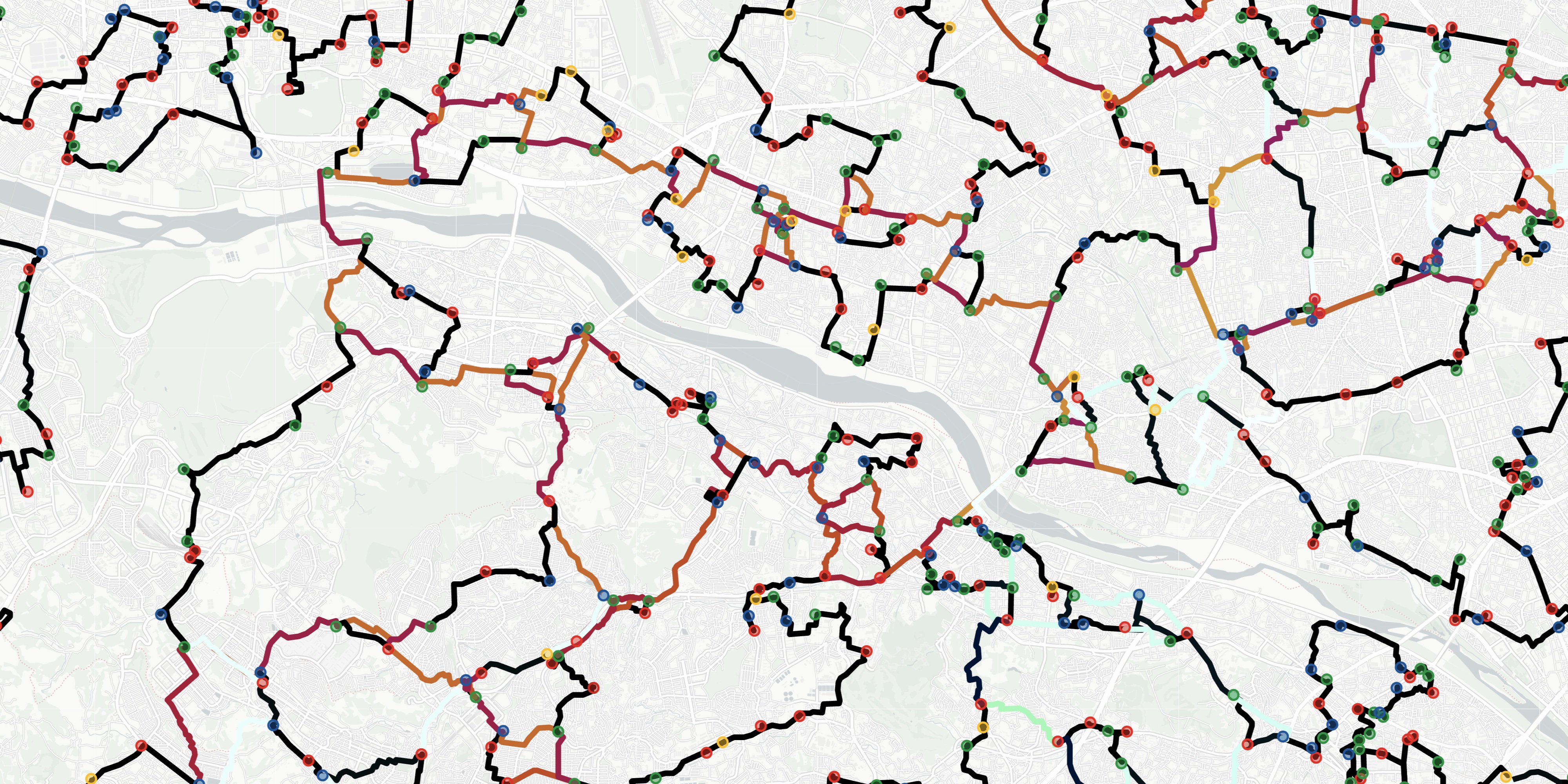
In the following two figures we display an LP solution we obtained for konbini40426. In the drawing, links are colored with a hue that gradually shifts from white to red to black for LP values ranging from 0 up to 1. Links of value 0 are colored white (to keep the image uncluttered, we do not draw links having value less than 0.01), links of value 0.5 are colored red, and links of value 1 are colored black.
You can see in the full-Japan image that many of the edges are black, meaning the LP rules we added have done a good job restricting the values assigned to links. But there are colorful regions, such as in the second image, where more work is needed. In our computation, we combine the cutting-plane method with a branch-and-bound search to handle these regions of the LP solution.
A branch-and-bound search attempts to increase the value of the lower bound by repeatedly splitting the set of candidate tours into two smaller sets. For example, we might chose a link between two stops and split the remaining tours into those that definitely use the link and those that definitely do not use the link. We thus create two new child subproblems from a single parent. Applying the cutting-plane method to each child, we can possibly improve in each case the LP bound given by the parent, and thus increase our overall lower bound.
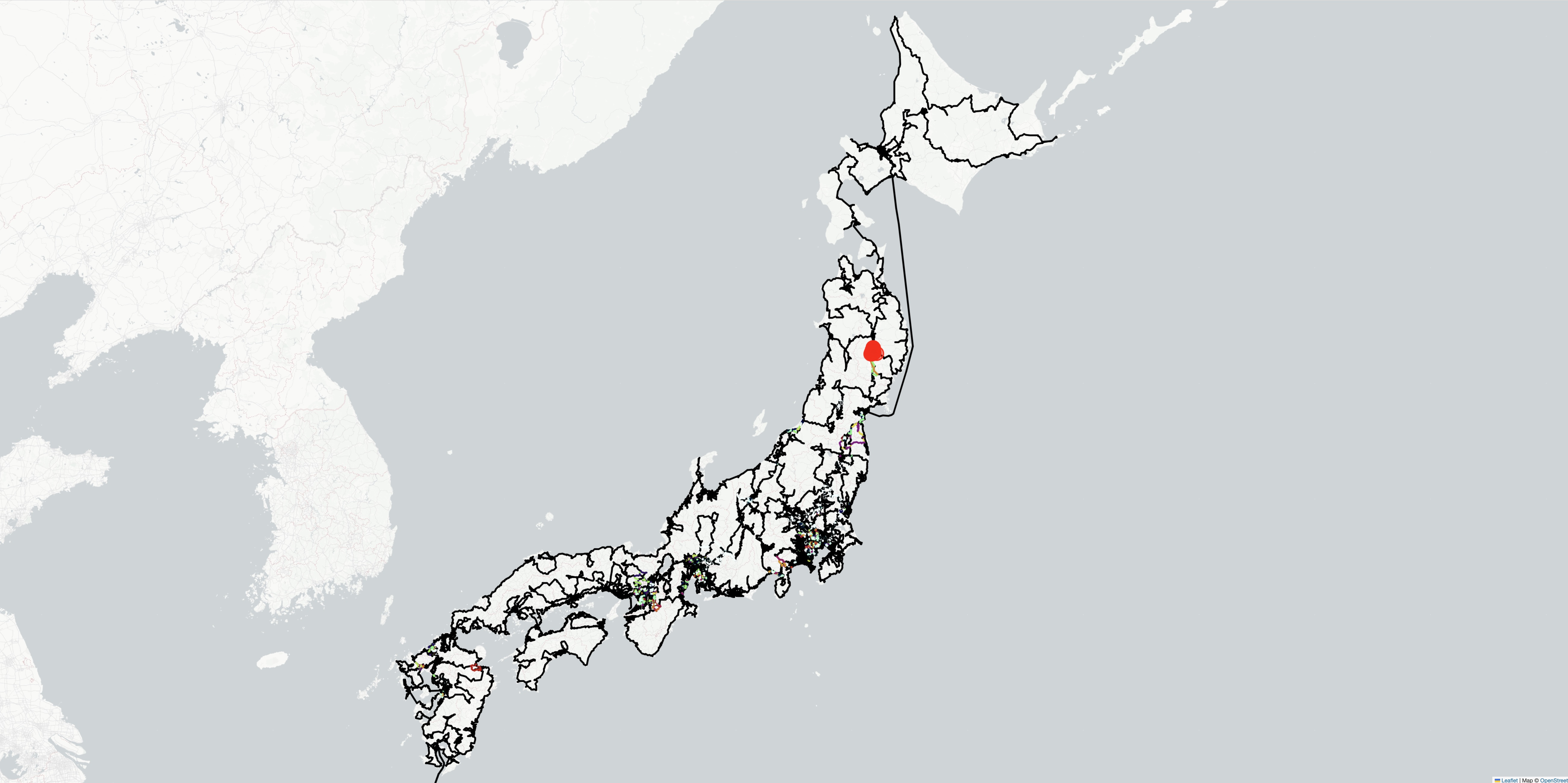
In the full-Japan image below, we display an optimal solution for an LP model that provided a lower bound β = 35574287. This is a strong LP model. It assigns 26347 links the value 1 and gives a gap of only 4147 seconds between the lower bound and the 35578434 tour length. Nonetheless, a branching step can improve the bound.
For this LP model, Concorde selected to branch in the region highlighted in red in the full-Japan image given below. This region of the LP solution is expanded in the second image, where a set of stops is indicated by the blue disk.
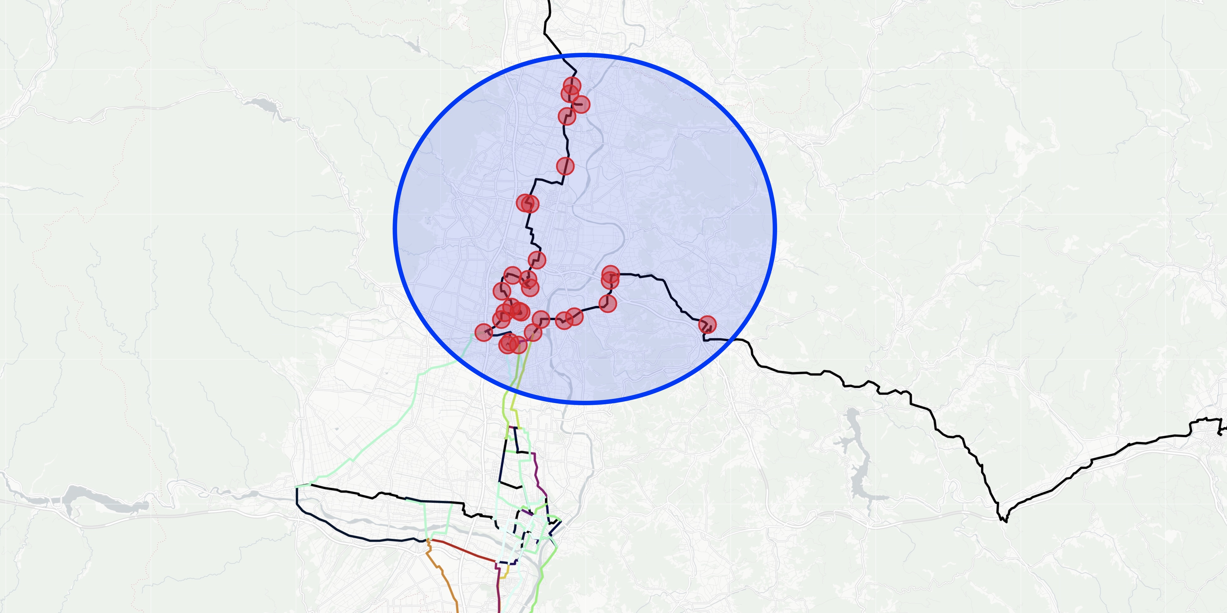
The links having one end in the indicated set and the other end not in the set sum to 2.8. This is ideal for branching, since a tour must go in and out of the set an even number of times. We split the problem into two child subproblems, one subproblem having the constraint that the links going in and out of the set must sum to at most 2 and the second subproblem having the constraint that the links going in and out of the set must sum to at least 4. Adding cutting planes yields a bound of 35577076 for the first subproblem and a bound of 35576908 for the second subproblem. Since any tour must be a candidate LP solution for one of the two subproblems, we now know that any tour must have length at least 35576908. The branching step improves the gap from 4147 seconds down to 1526 seconds. And we can continue the process by branching in each of the subproblems.
A nice side-effect of a branch-and-bound search is that the process can identify cutting planes that can improve the initial LP model. This gives the possibility to restart the search from a better model. In the table below we display results from such repeated runs for konbini40426. You can see in the "LP Bound" column the value given by the LP model used to initiate each successive branch-and-bound search. The TSP was finally solved in the 5th run, using a total of 113,651 subproblems.
| Run | LP Bound | B&B Bound | Gap | Subproblems | Core Years |
|---|---|---|---|---|---|
| 1 | 35569297 | 35578030 | 404 | 18301 | 1.9 | 2 | 35571235 | 35578286 | 148 | 119463 | 4.9 |
| 3 | 35573063 | 35578054 | 380 | 809 | 0.2 |
| 4 | 35573649 | 35578328 | 106 | 47915 | 11.8 |
| 5 | 35574032 | 35578434 | Optimal | 113651 | 23.4 |
| 6 | 35574287 | 35578246 | 188 | 871 | 1.9 |
| 7 | 35574350 | 35578199 | 235 | 1101 | 0.9 |
| 8 | 35574368 | — | — | — | — |
Even after solving konbini40426, we continued to study the problem with 3 additional runs, always looking for stronger LP-bounding techniques.
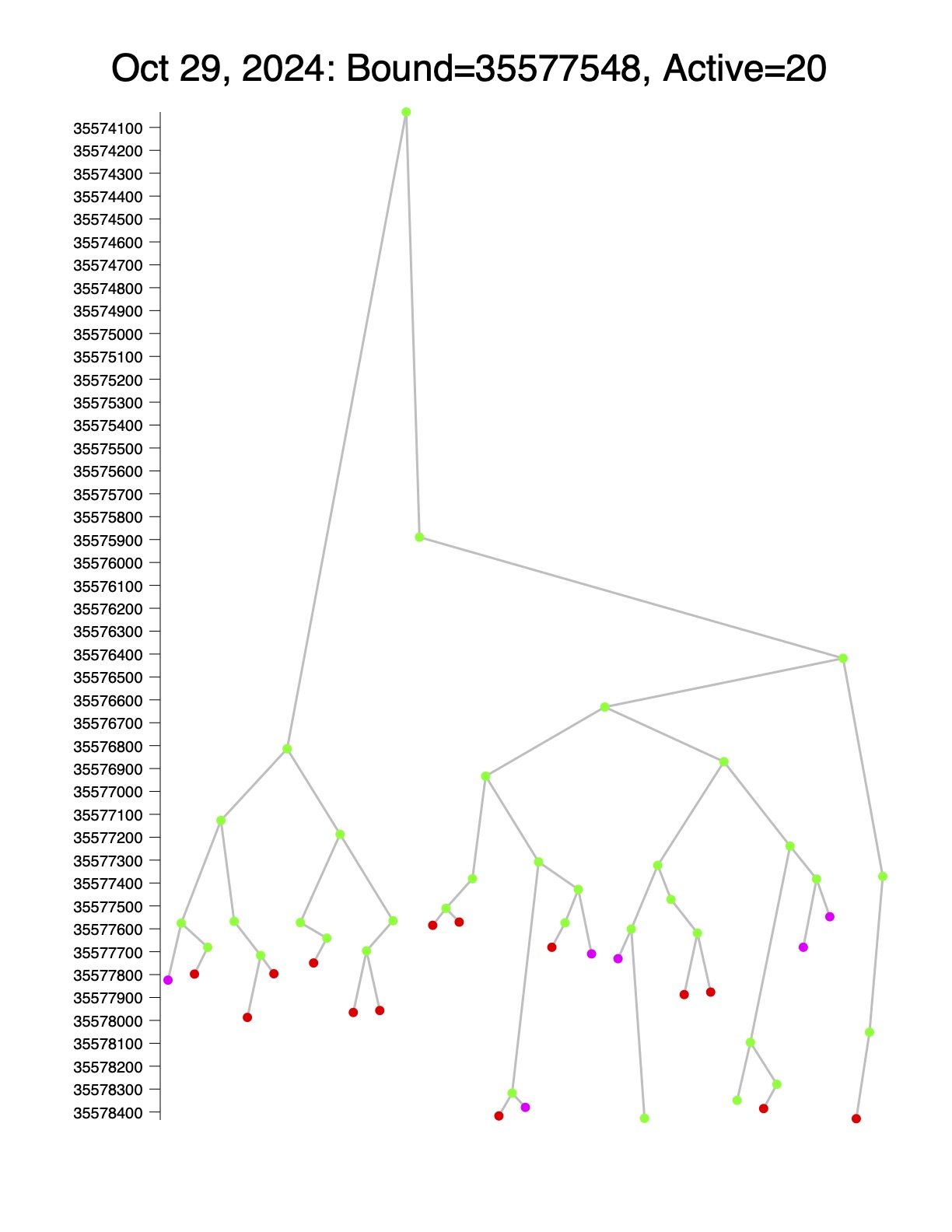
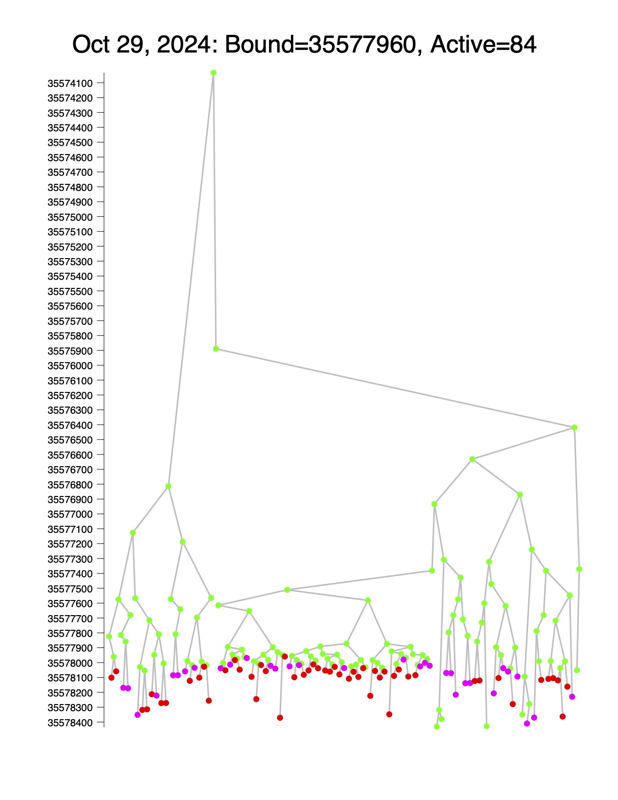
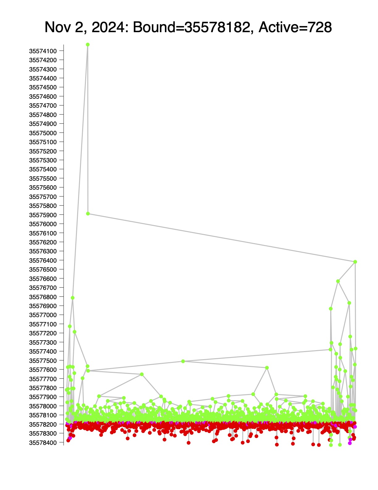
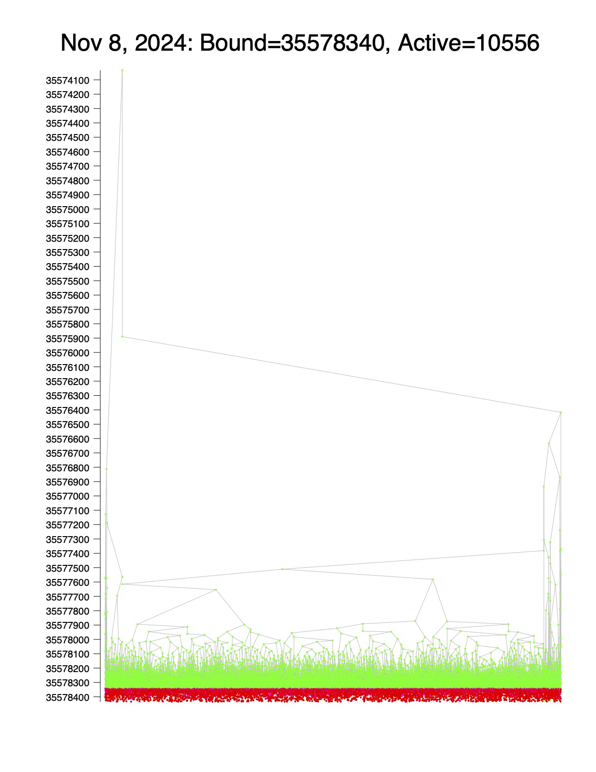
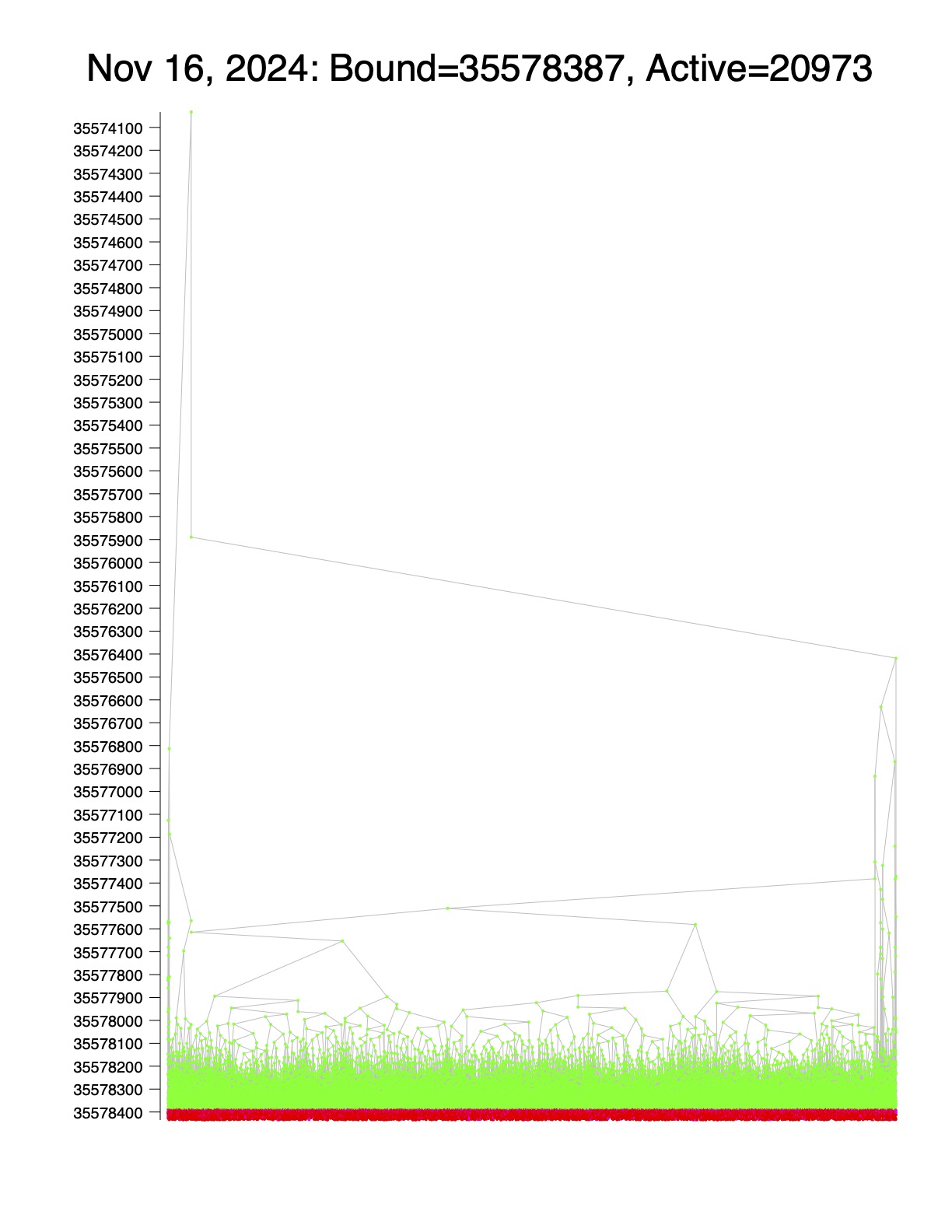
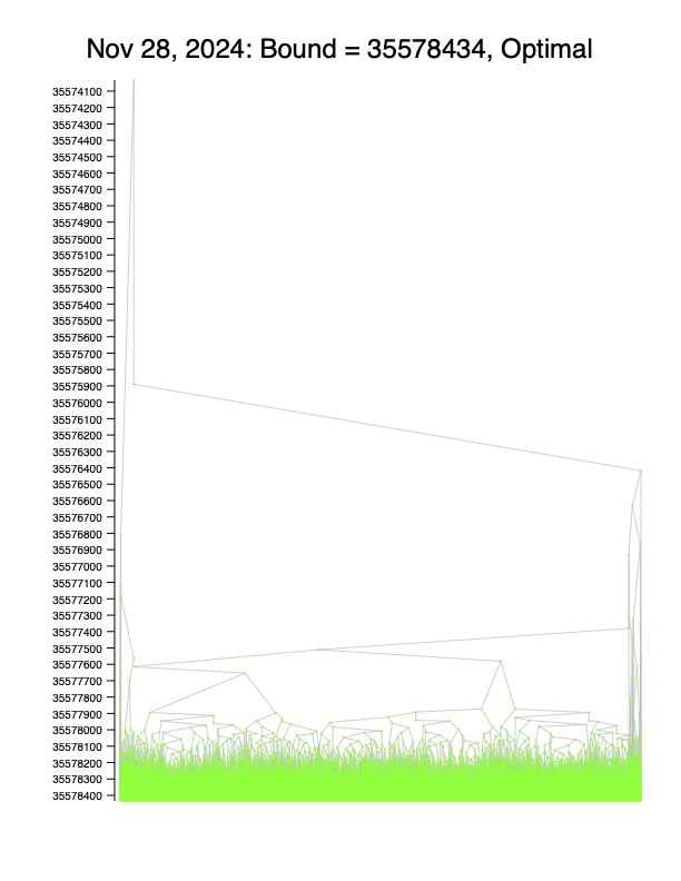
The images below are snapshots of the branch-and-bound search (Run 5) used to solve konbini40426, each depicting the search tree on the indicated date. The active nodes of the trees (those representing subproblems that have not yet been processed) are colored either red or magenta. The red nodes are those that have not yet gone through additional rounds of the cutting-plane procedure after the branching step. The height of a node indicates the optimal value of its LP relaxation.
At the top of each image, we display the lower bound established by the search and the number of active subproblems. Notice the red/magenta line of active nodes slowly moving down the images, as the search progresses to better and better lower bounds.
Click on the images to see high-resolution versions.
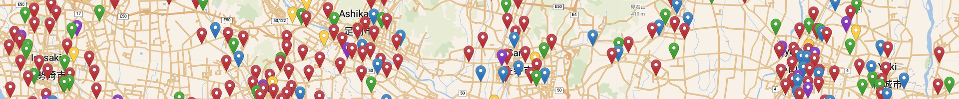
The tour map-drawings were created with the Leaflet open-source JavaScript library for mobile-friendly interactive maps and make use of map tiles built by OpenStreetMap, by Carto Basemaps and by Stadia Maps.