An Amazon driver's day begins at a depot or warehouse, where she/he loads a van with customer packages to be delivered to homes in an assigned neighborhood.

Although not part of the Last Mile Routing Research Challenge, the processes involved in getting a depot full of packages sorted into loads for individual vans (think knapsack problem) are certainly interesting and difficult in their own right. But in the routing problem considered here, we assume we have a driver, a loaded van, and a full tank of gas, ready to roll.
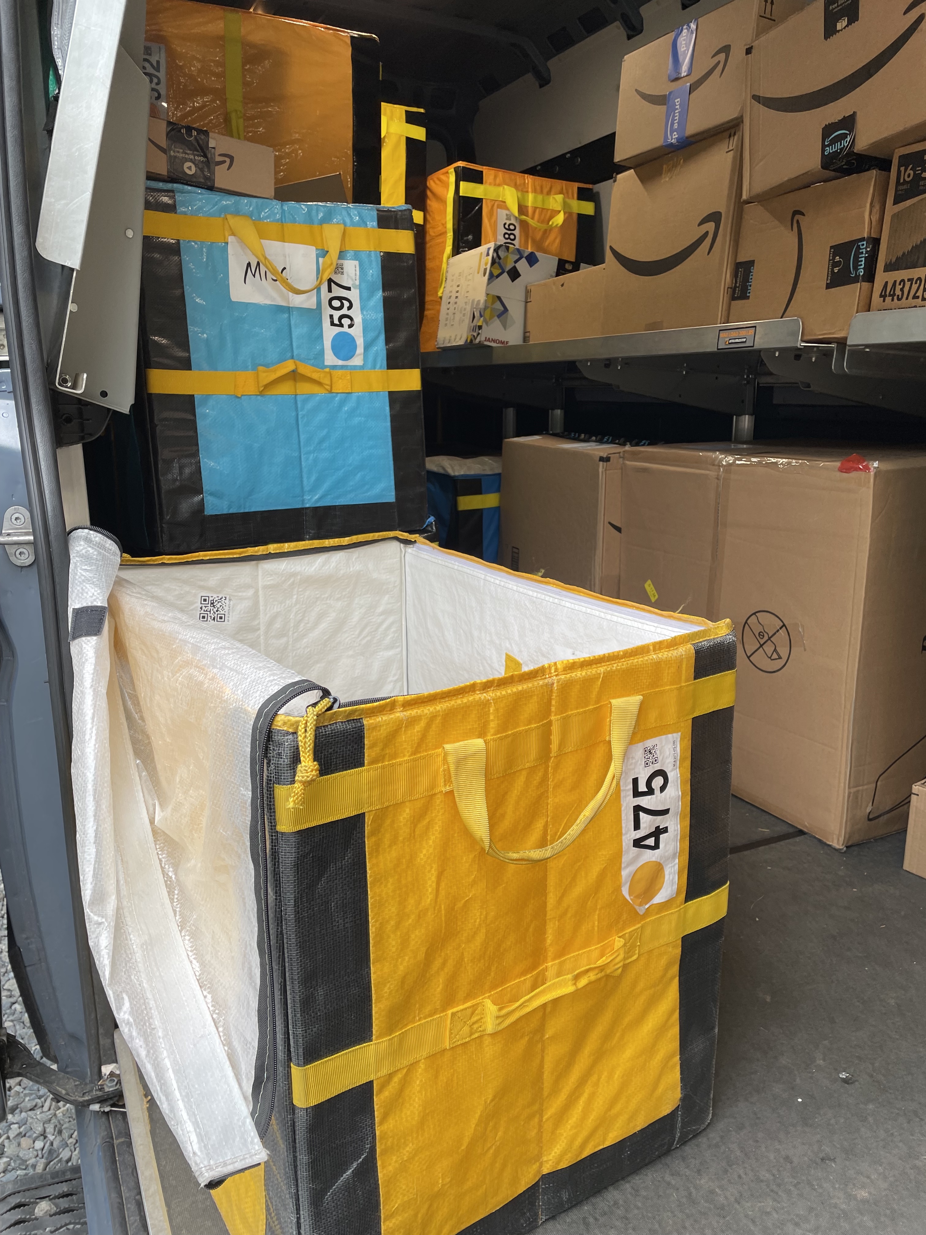
I should add that, despite the sometimes comically overloaded vans you can see in posts on the Amazon DSP Drivers section of reddit.com, the vans I've noticed outside our house are typically well organized by the driver. Smaller packages are arranged in large (collapsible) bags along the walls and oversized packages line the floor and upper racks. The bags play a roll in our proposed solution method for the routing challenge.
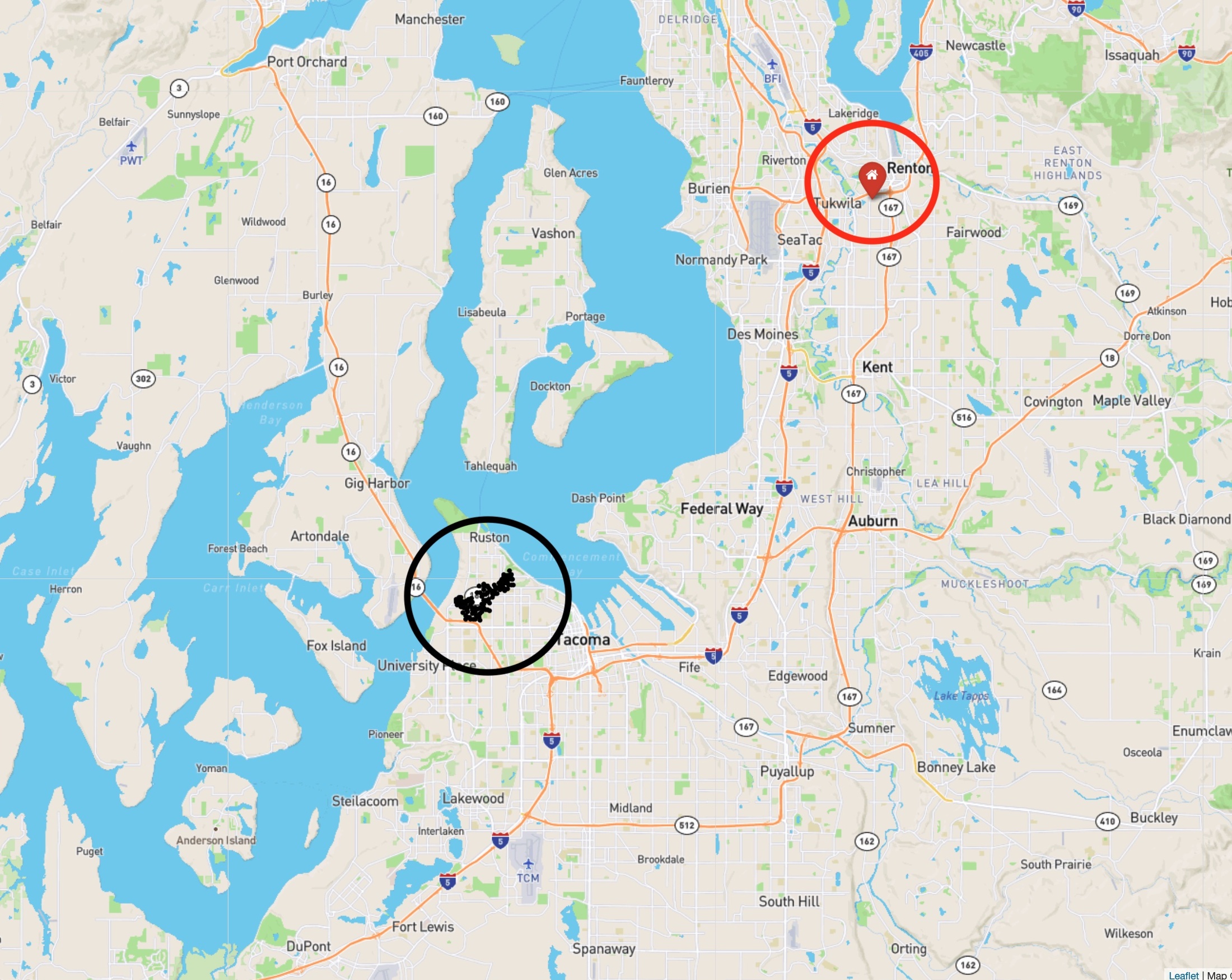
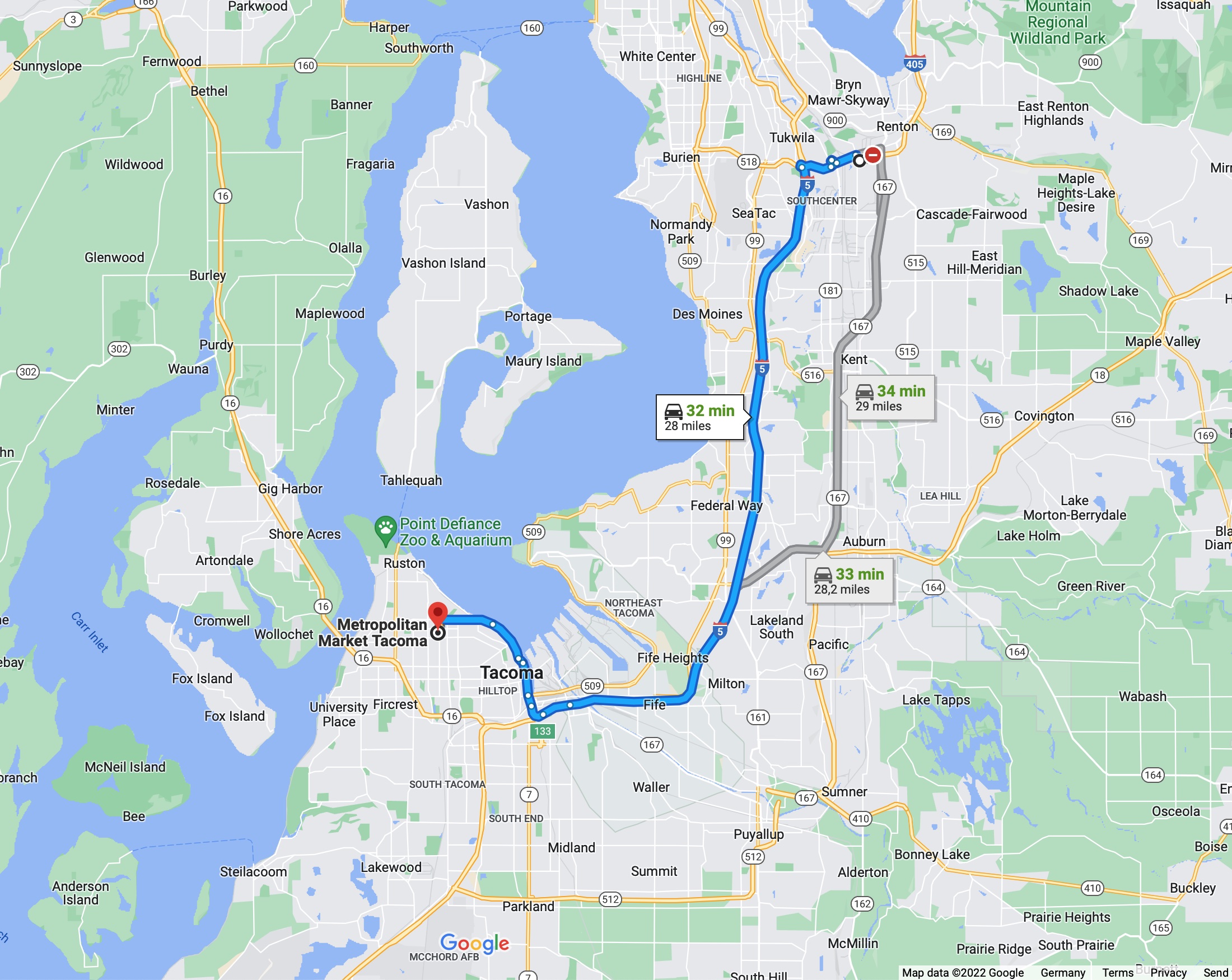
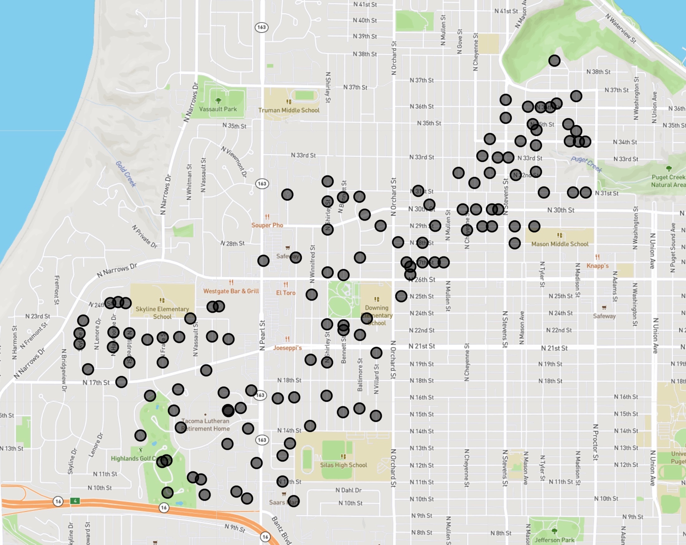
An example of the routing problem faced by Amazon's drivers is illustrated in the three images below. The route begins at the DSE5 depot in Renton, WA, indicated by the red marker inside the red circle. The customer neighborhood to be served is indicated by the black points in the black circle. It is an easy matter to use Google Maps to find the shortest path from the depot to the neighborhood, zipping down Interstate 5. The real task is to find an efficient way to visit the actual customer stops, indicated by the black disks in the third image, showing house locations along the grid of streets.
Routing the van to each of the stops is an instance of the asymmetric traveling salesman problem (ATSP). The asymmetry is that the time to travel from stop X to stop Y may not be the same as the time to travel from Y back to X, due to one-way streets, left-hand-turns, and other traffic considerations. This particular instance has 127 stops plus the depot, so a 128-point ATSP.
A reader of the popular science press might throw up their hands at this point.
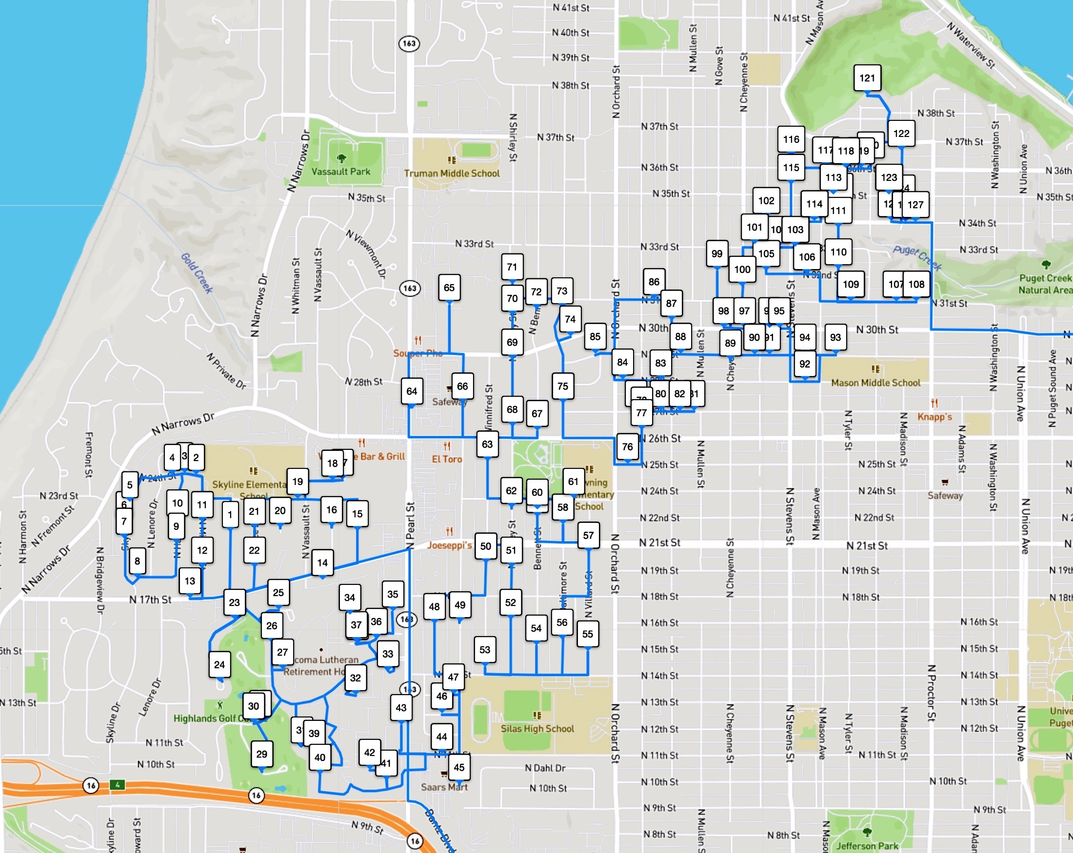
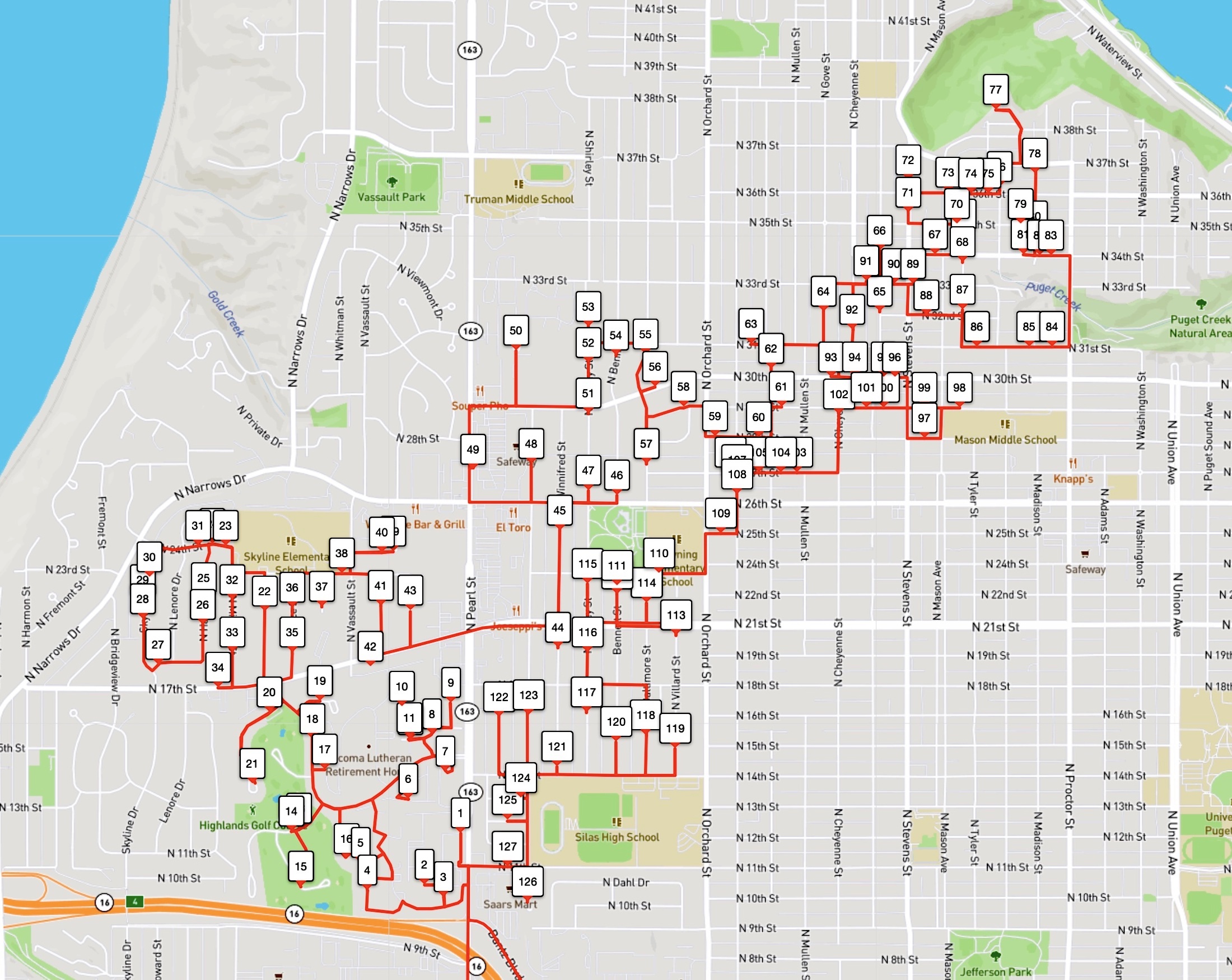
And indeed, the route followed by the driver in this example is not shortest possible. The driver tour is indicated in the first image below, while the optimal tour is given in the second image. Using the Amazon-supplied point-to-point travel times, the driver tour clocks in at 12431.3 seconds and the optimal tour takes 11788.4 seconds. So it would be possible to cut down the driver's road trip by about 10.7 minutes. (On average over the 1,107 Amazon test instances we consider, the saving is actually over 23 minutes, making a good argument for a longer lunch break.)
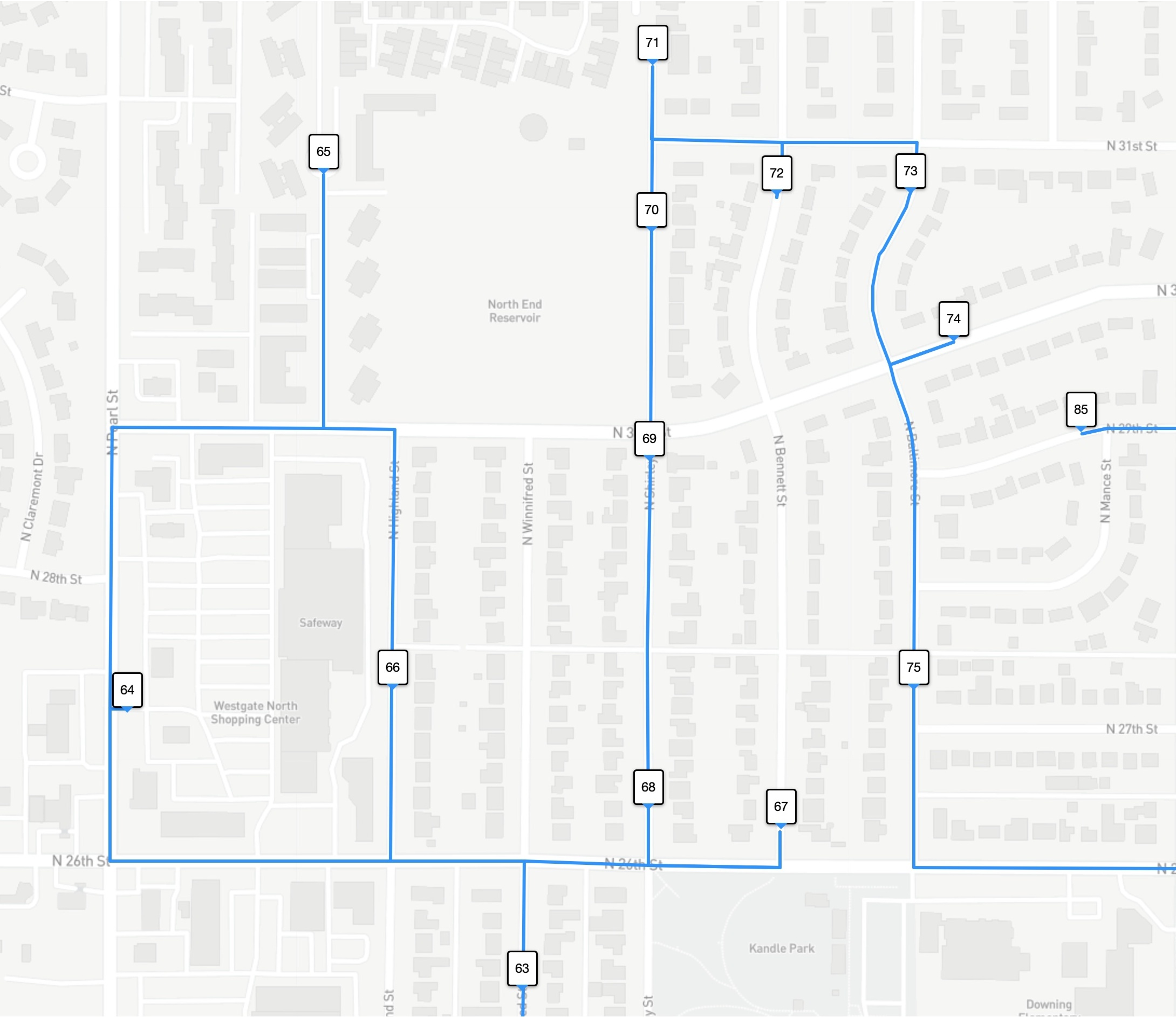
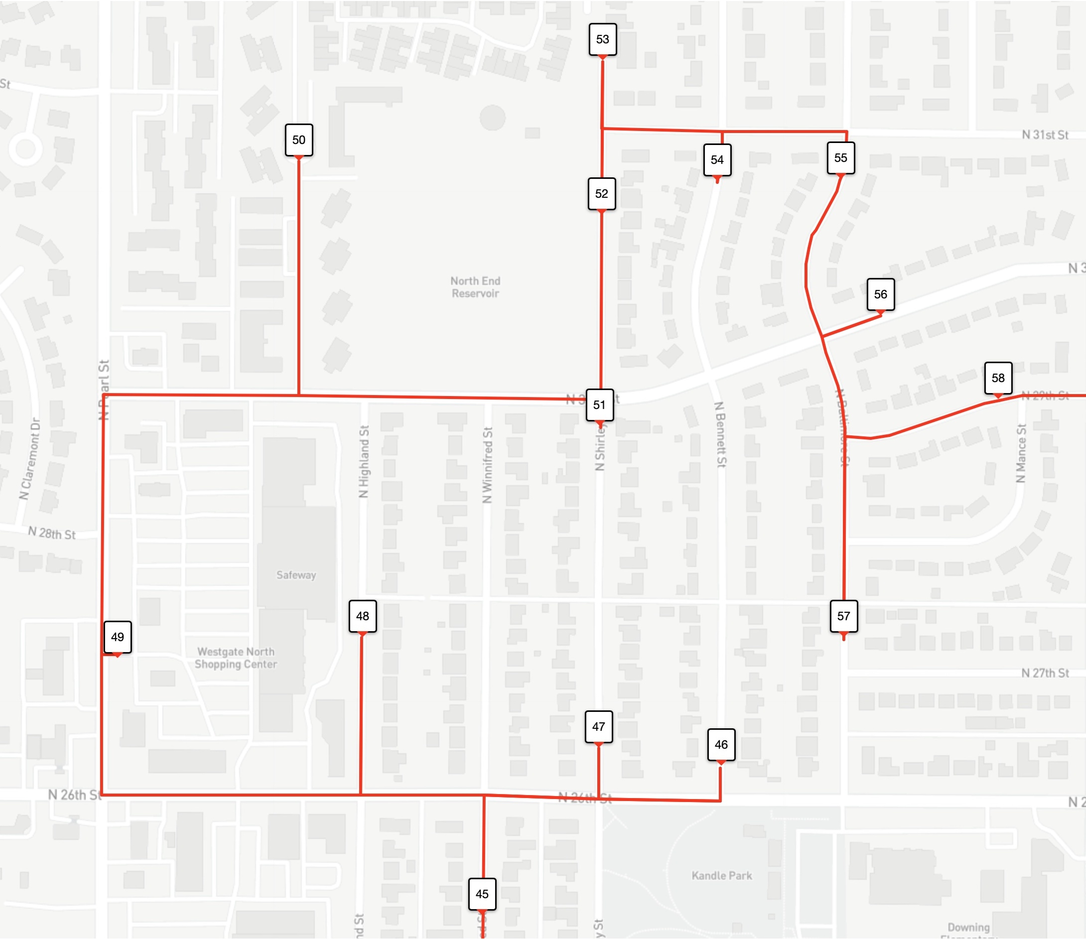
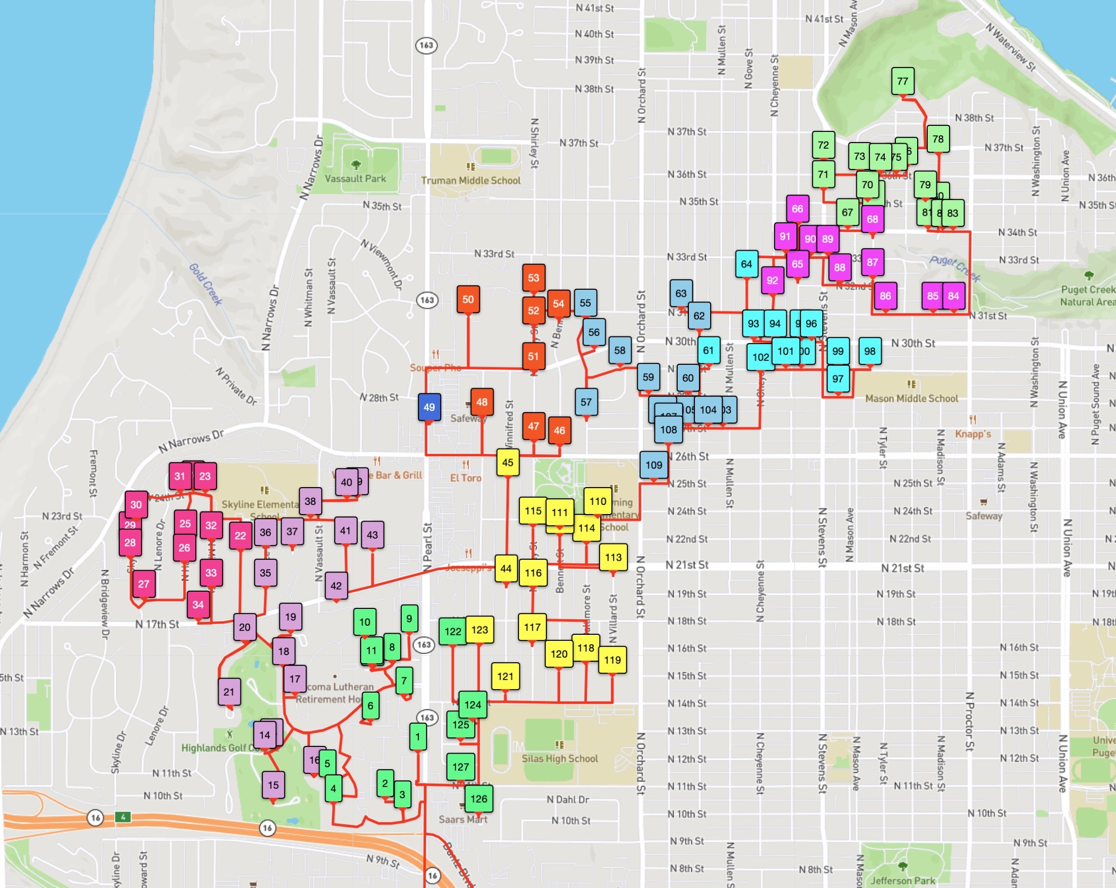
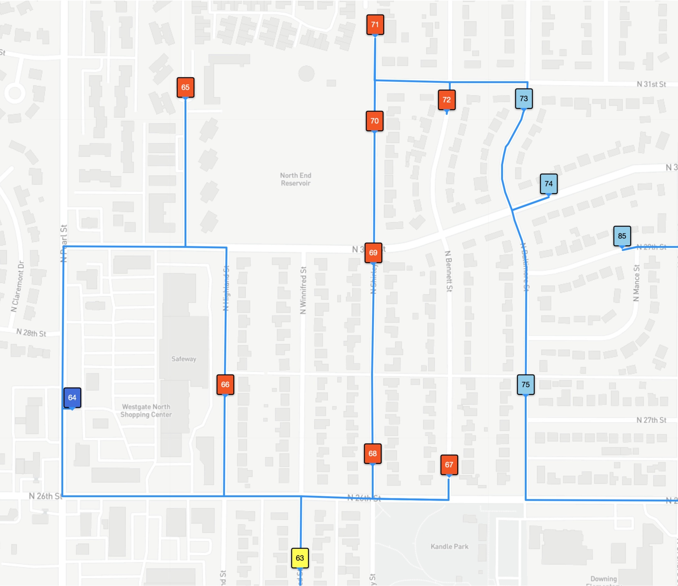
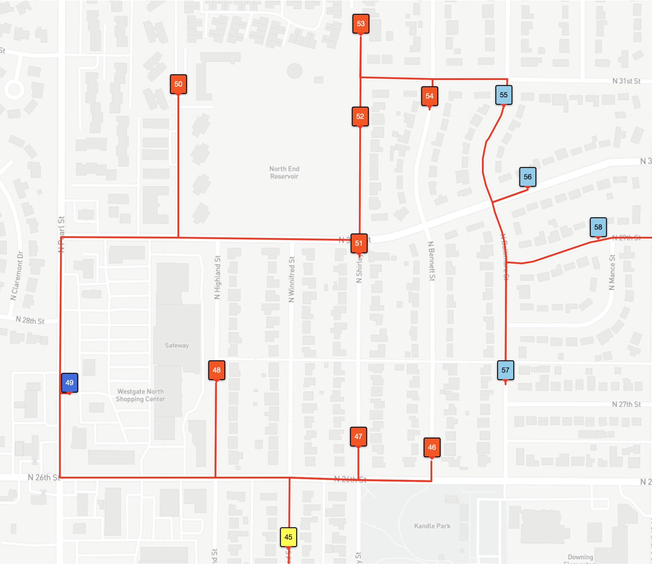
With so many stops, it's difficult to see that the optimal tour is actually shorter than the driver tour. But if we zoom in on the North End Reservoir, you can see that the optimal tour (the one in red) visits the stops in a more efficient path. In our images, the stops are numbered by the order they are visited by each tour.
This raises two questions. The first is that you're killing me bro. How are you claiming to have the shortest-possible tour for this instance of the ATSP? This one is easy: the popular press is greatly overstating the difficulty of solving a modest-sized practical instance of the traveling salesman problem. This 128-point instance was handled in 7 minutes on a single-processor workstation. (On the 1,107 Amazon test instances, the average running time was 142 seconds.) If you are interested in seeing the techniques used in the computation, please have a look at the talk Optimal Tours given at the National Museum of Mathematics in August 2021.
The second question is that if the TSP is so easy, why aren't Amazon and the van driver using an optimal (or at least a near-optimal) solution? That gets to the heart of the Last Mile Routing Research Challenge. Amazon's researchers know how to solve instances of the TSP. For example, if you are satisfied with near-optimal solutions, you can employ techniques such as those adopted in Keld Helsgaun's LKH code. (Actually, for these Amazon instances, LKH will typically find an optimal tour, but the design of the code does not provide a proof that the tour is optimal. So you might miss a few seconds on some examples.)
There can be many reasons why Amazon or Amazon's driver might prefer a non-optimal route. We discuss this aspect of practical routing on the Amazon Challenge page. Indeed, the stated goal of the challenge is not to find optimal tours, but rather to find tours closely matching routes taken by experienced Amazon drivers.
To set things up for challenge participants, Amazon and MIT made available a collection of 6,112 routes driven by van drivers in 2018. These training routes are concentrated in 5 metropolitan areas in the US: Austin, Boston, Chicago, Los Angeles, and Seattle.
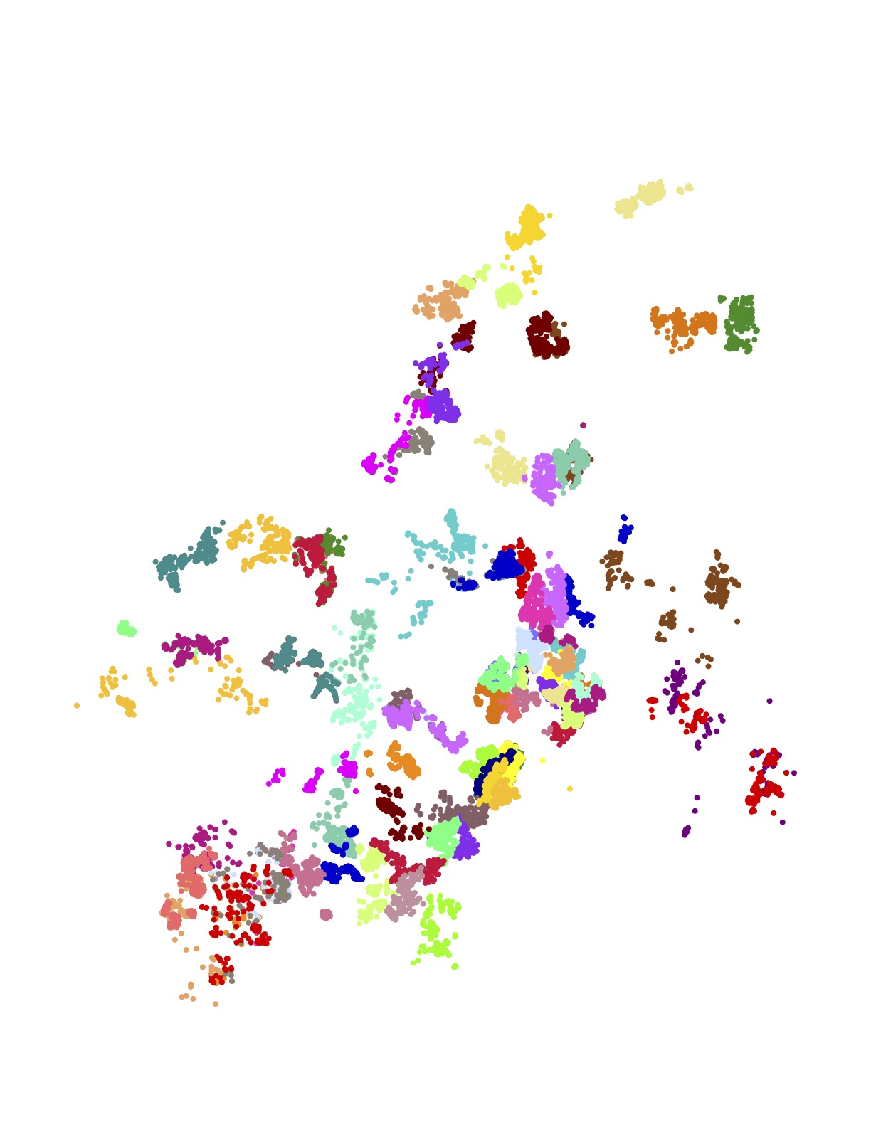
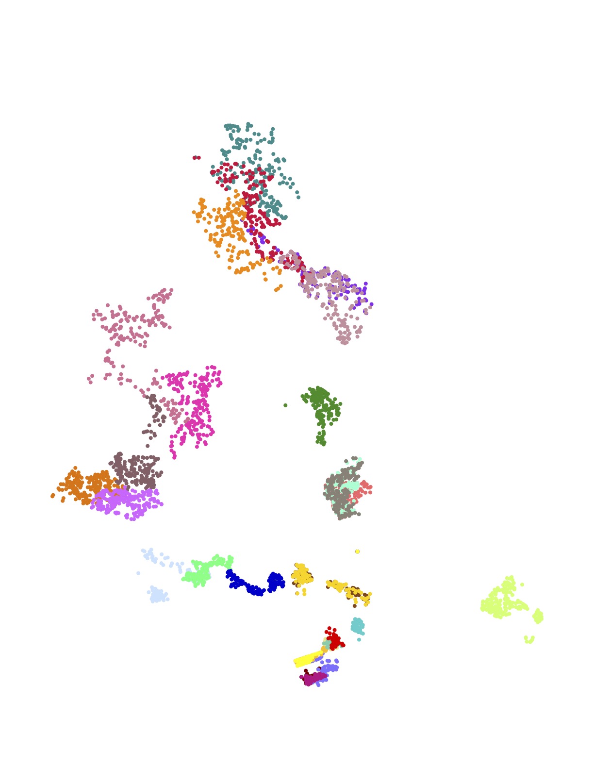
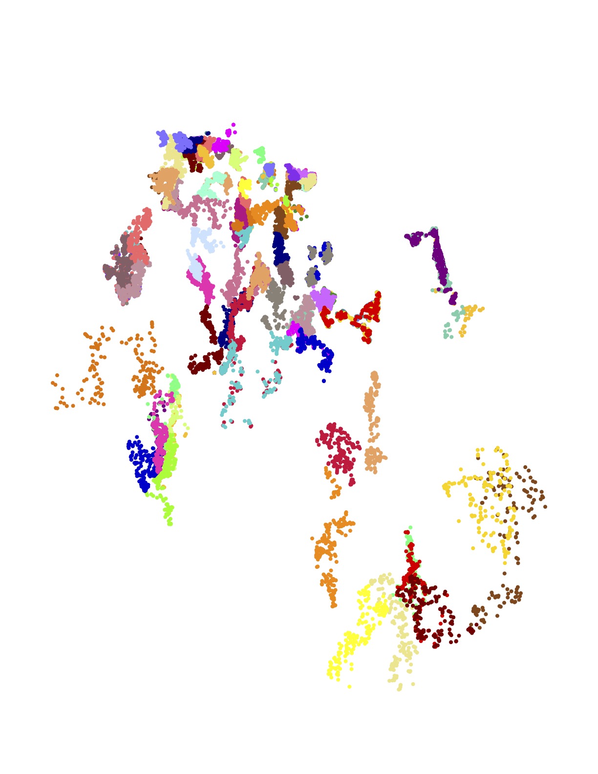
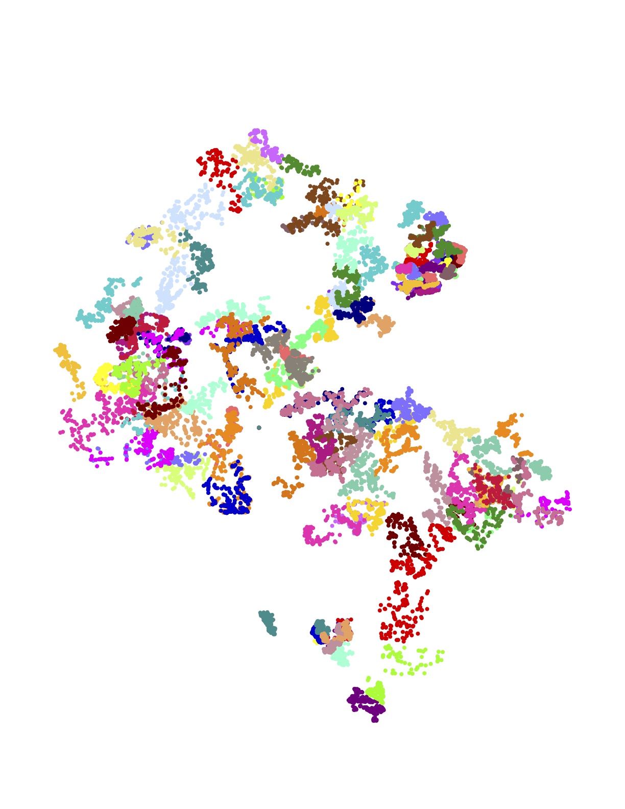
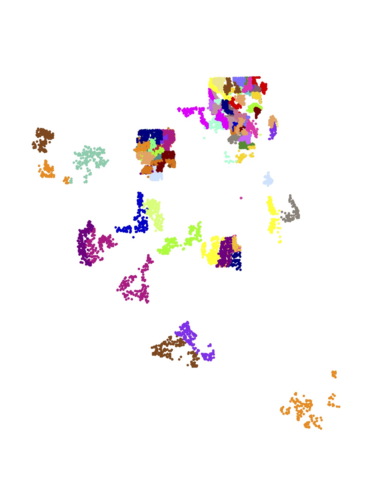
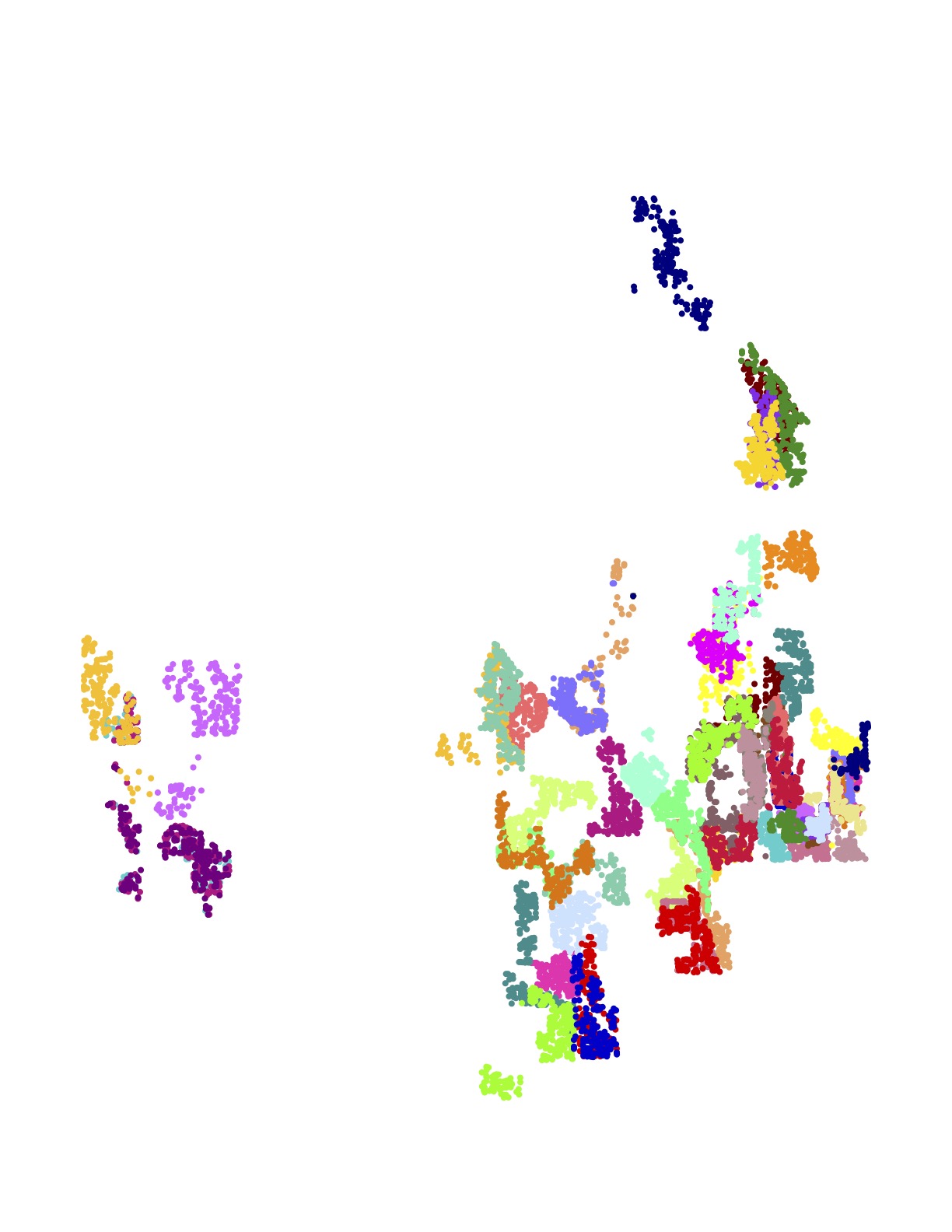
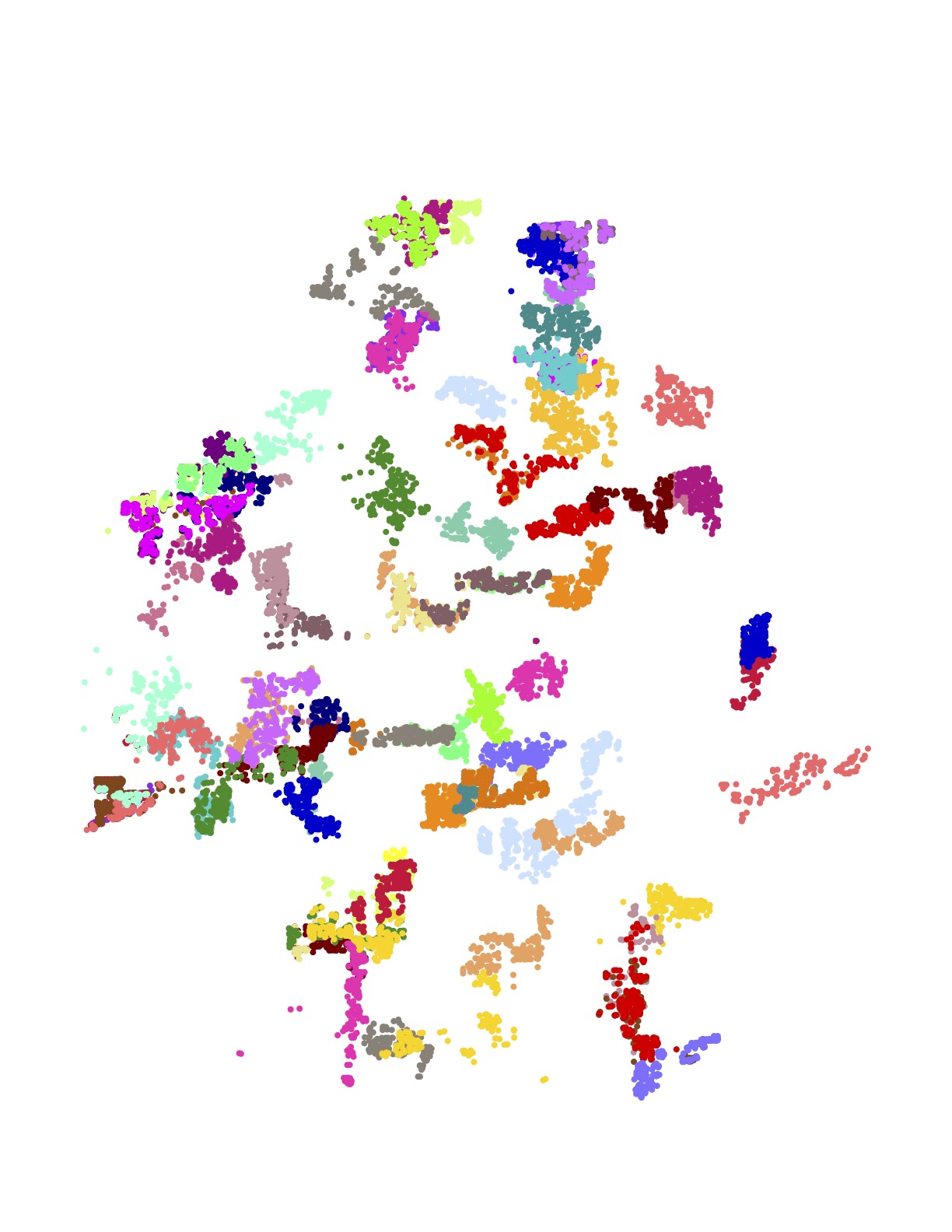
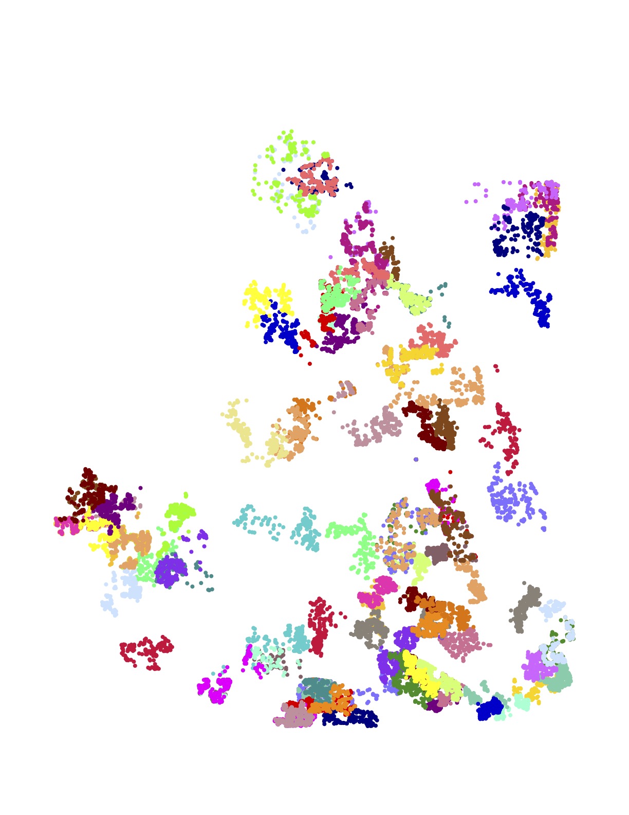
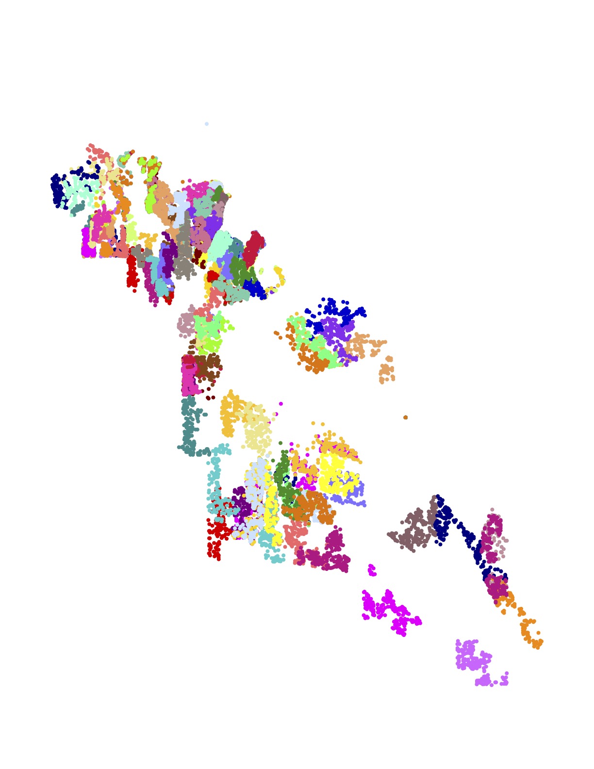
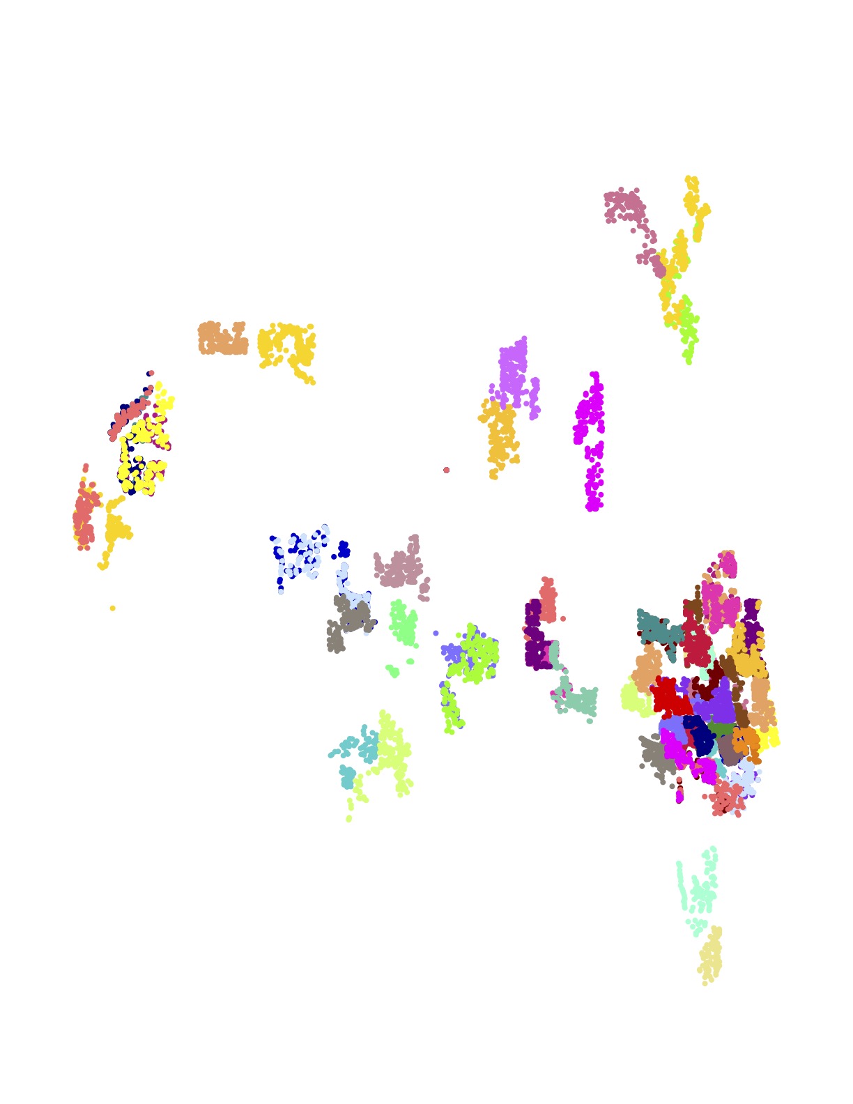
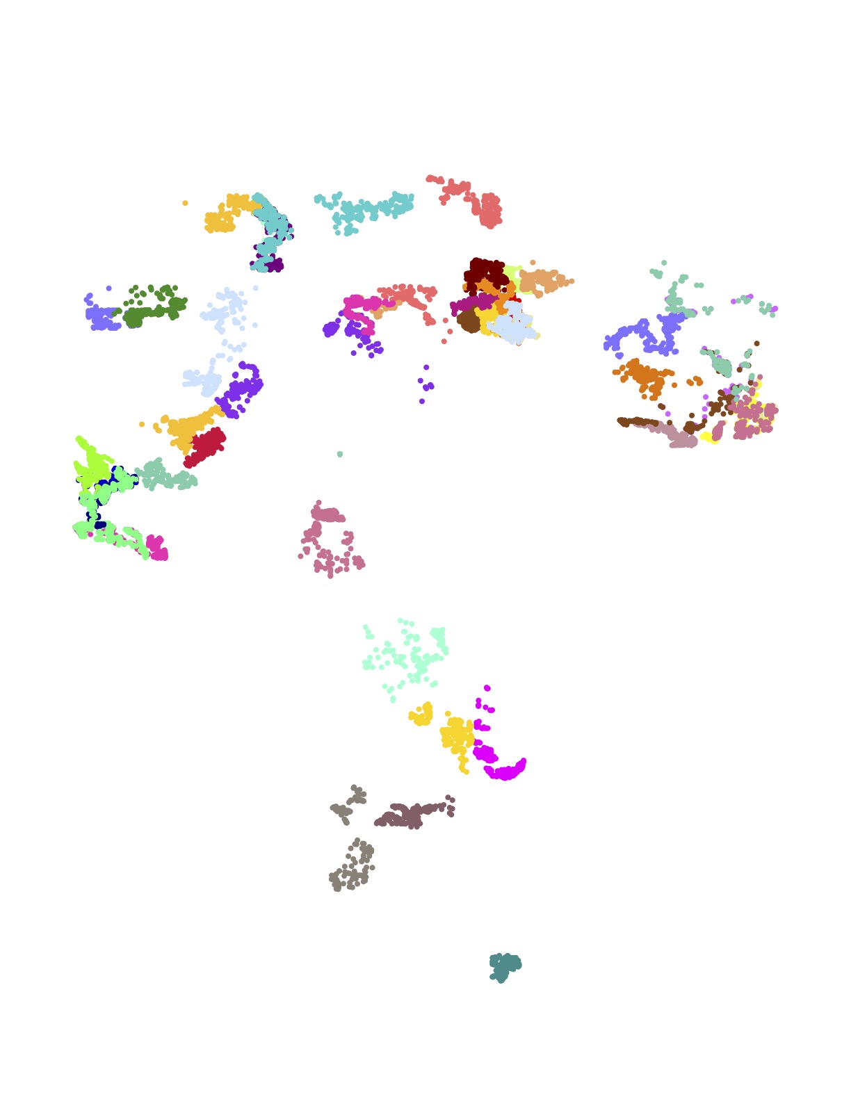
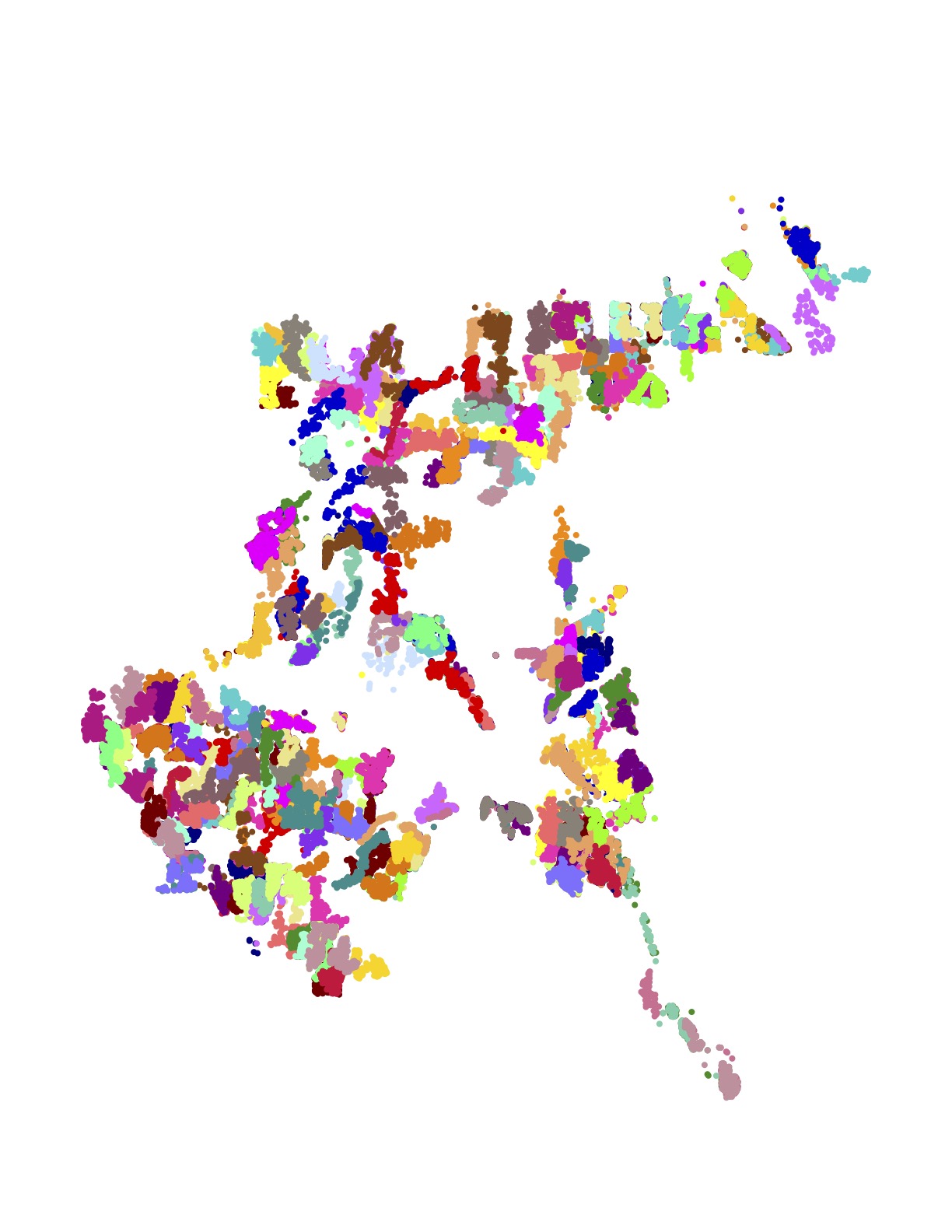
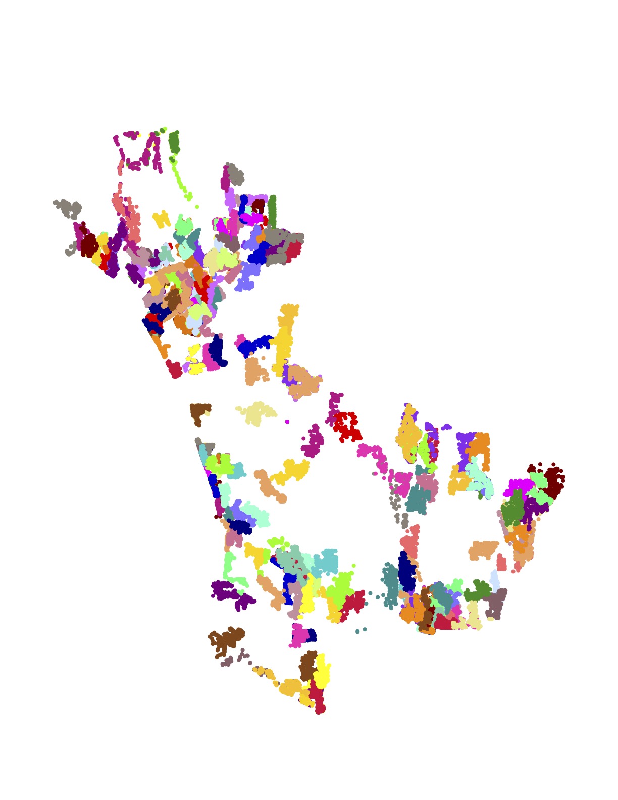
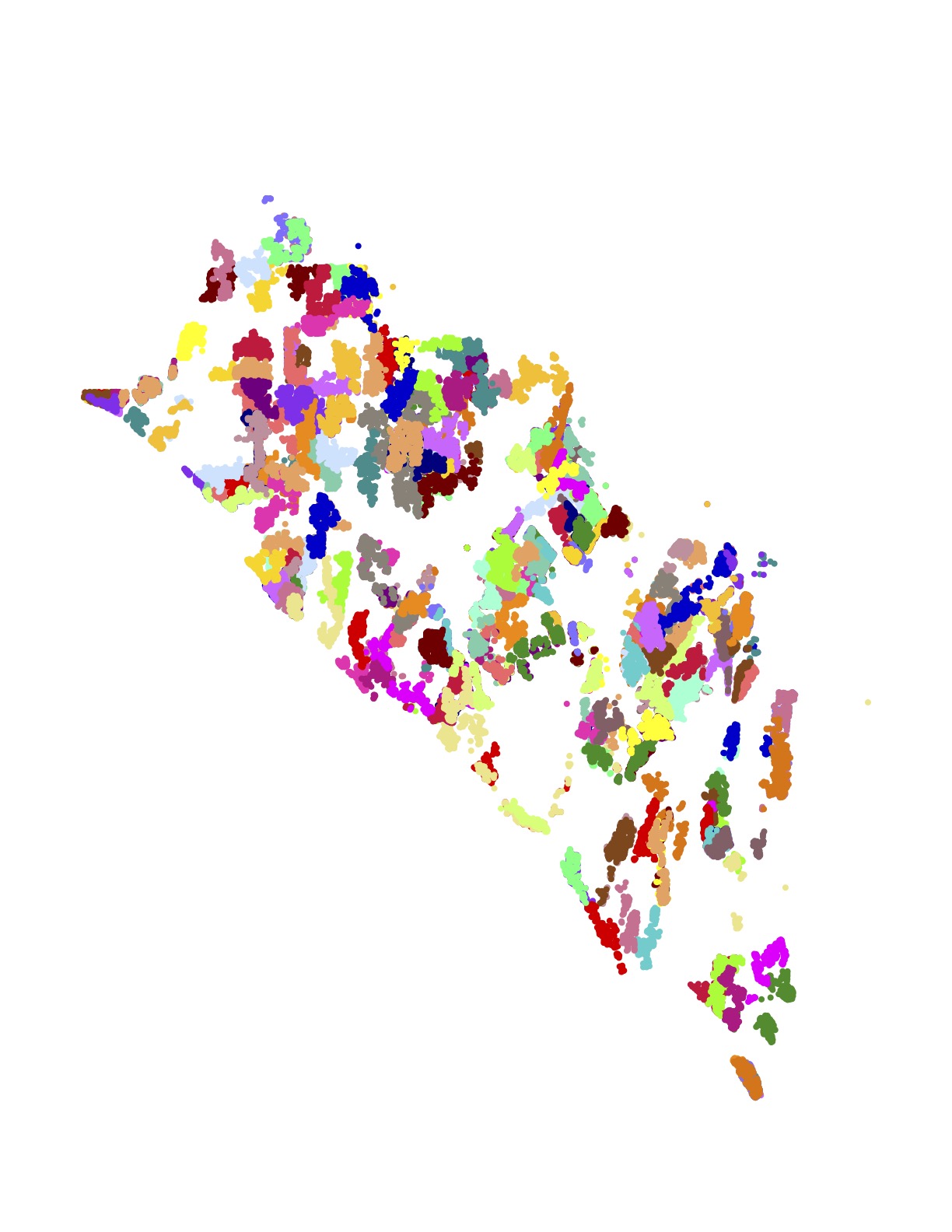
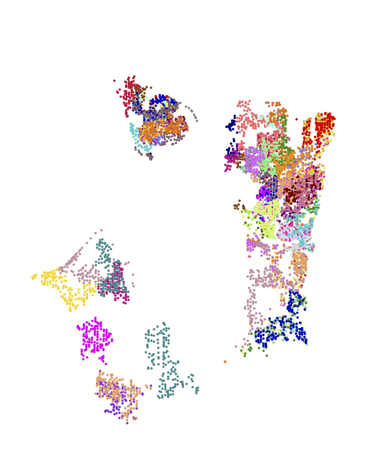
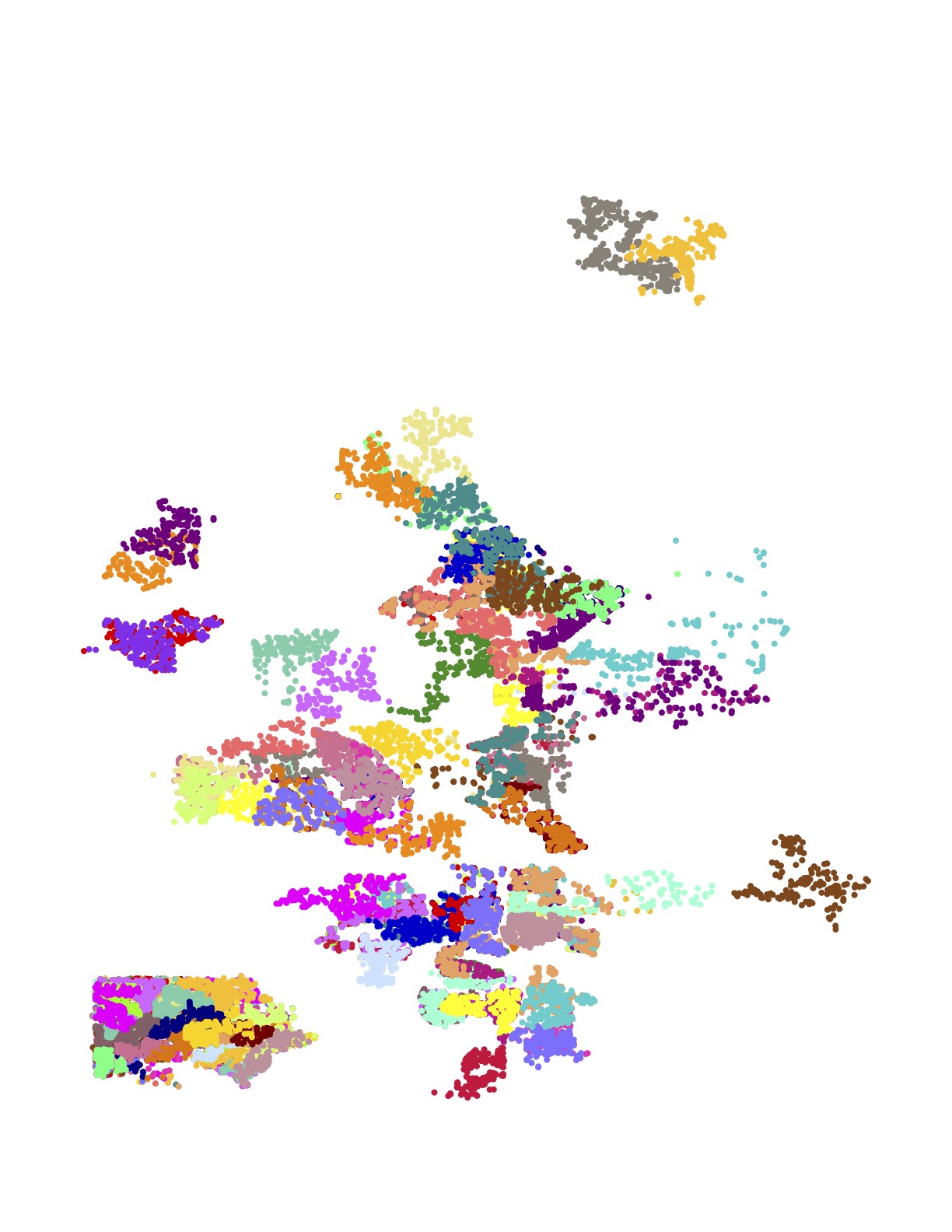
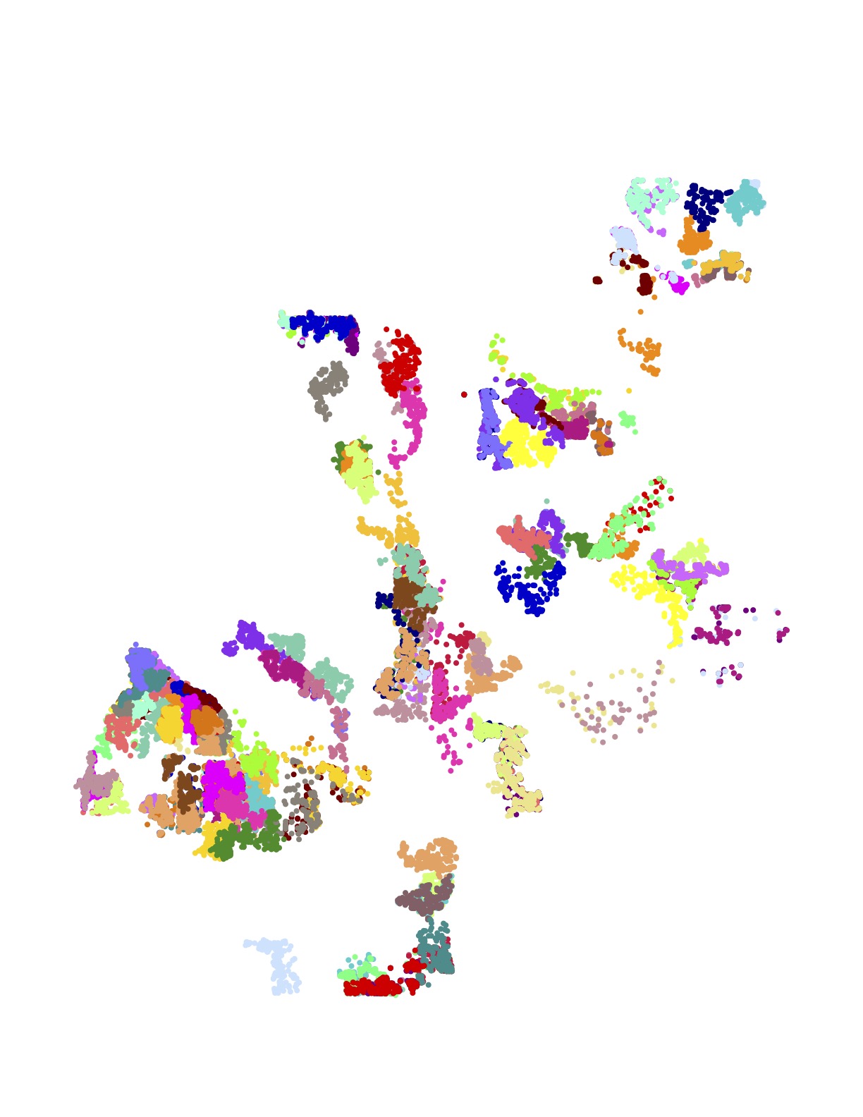
The following images present all 1,107 examples from the training set that are rated by Amazon as high quality driver tours and have no undelivered packages. These High+Delivered routes are the type that would be included in the scoring phase of the challenge. Each of the 17 images depicts the routes originating at a particular Amazon depot. The colors indicate the customer stops handled by each route.
The training set is in one sense huge: researchers have never before been given such a large collection of real-world TSP instances to study. But in another sense, made clear in the above images, the data is sparse. There is little overlap in the coverage of the routes — most of the neighborhoods are geographically disjoint and individual houses are seldom visited more than once.
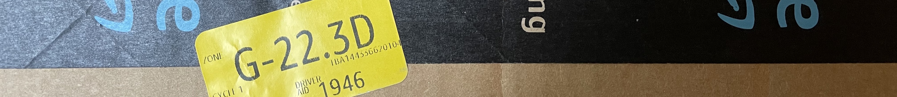
The ATSP tours are only a weak approximation of the driver sequences. For example, the optimal ATSP tour order does not reflect any conditions related to the warehouse operation or to the driver's storage of packages in the van she/he will be using that day. Regarding this, the training data provide a sort zone ID for each stop, indicating a possible clustering of the route's stops in a tour. You can see the sort zone IDs printed in a large font on the yellow stickers attached to packages arriving at your house.
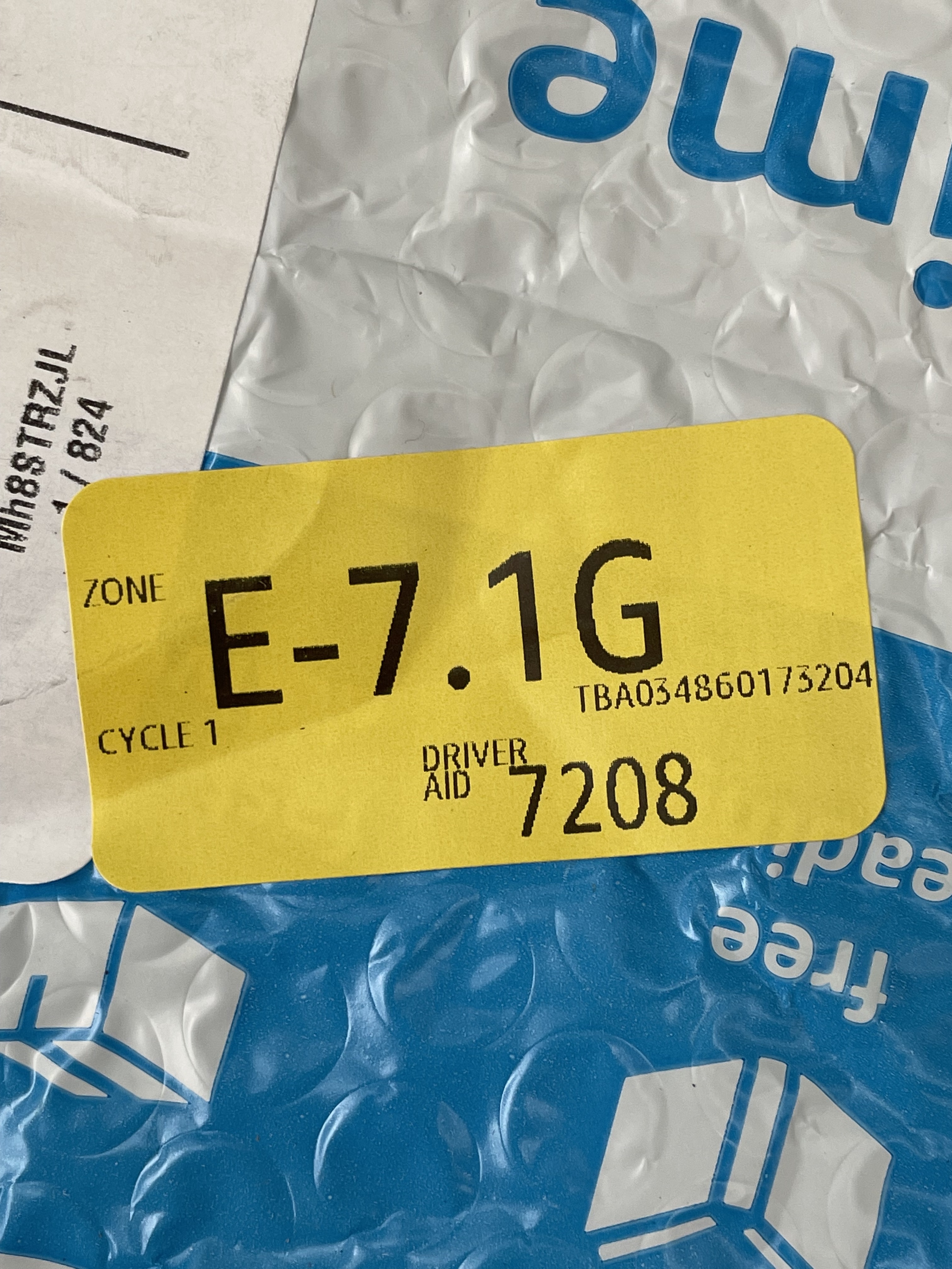
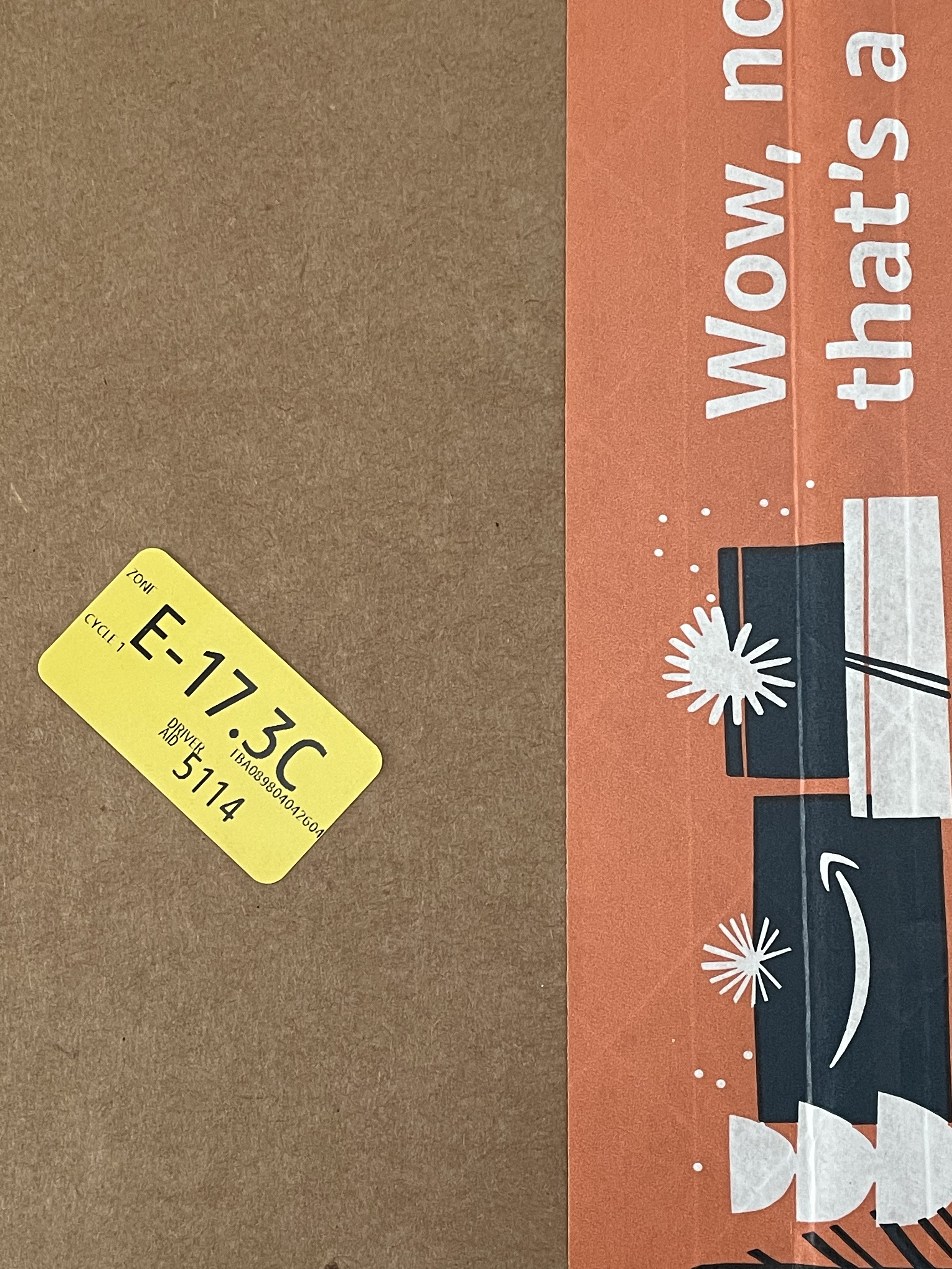
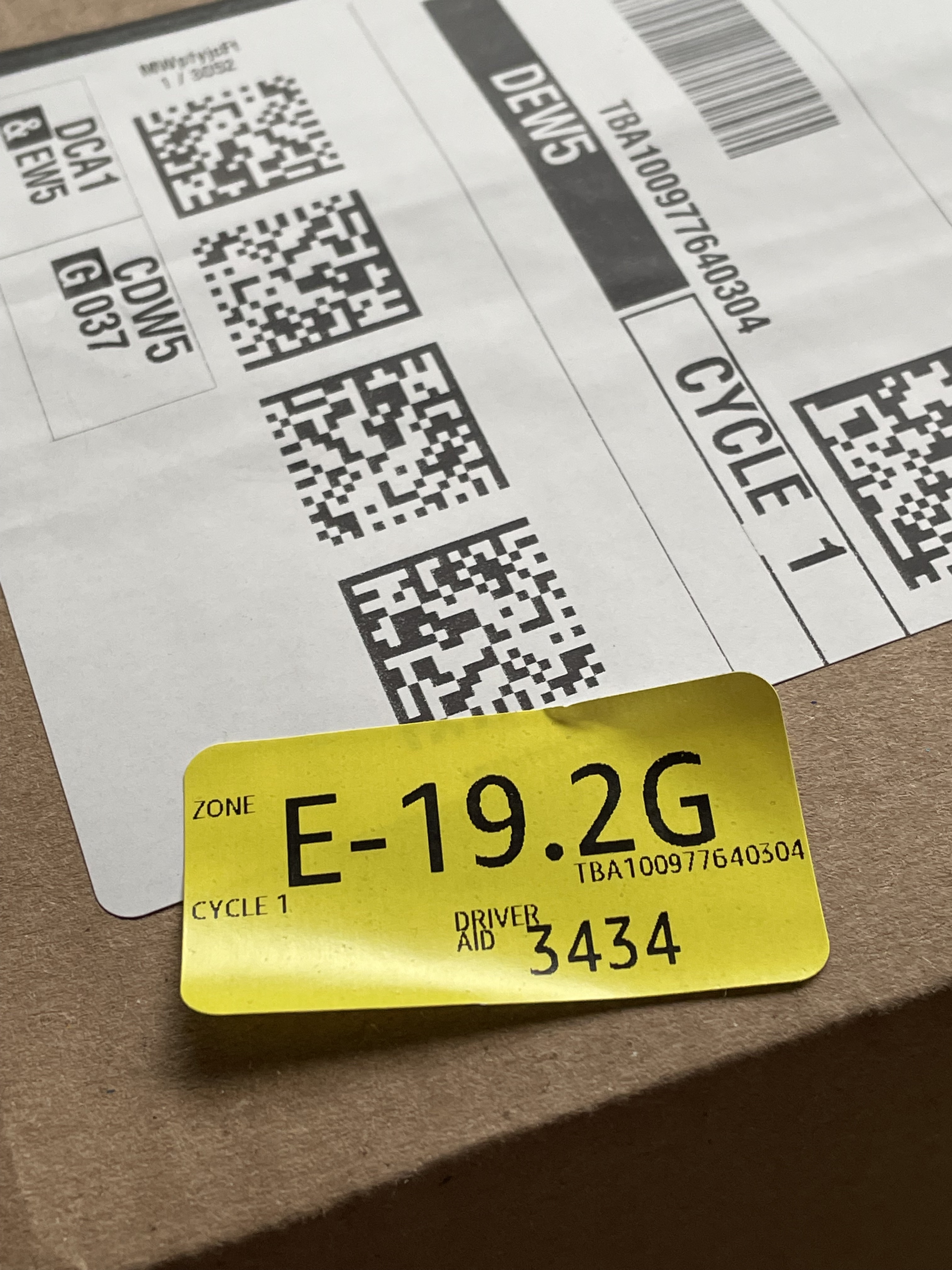
The three photos above are from packages that arrived at our home in New Jersey. You can see that the IDs are similar, but not identical. It appears that the sort zone IDs are assigned by Amazon on a daily basis, rather than having a fixed ID corresponding to the geographic location of the customer stop.
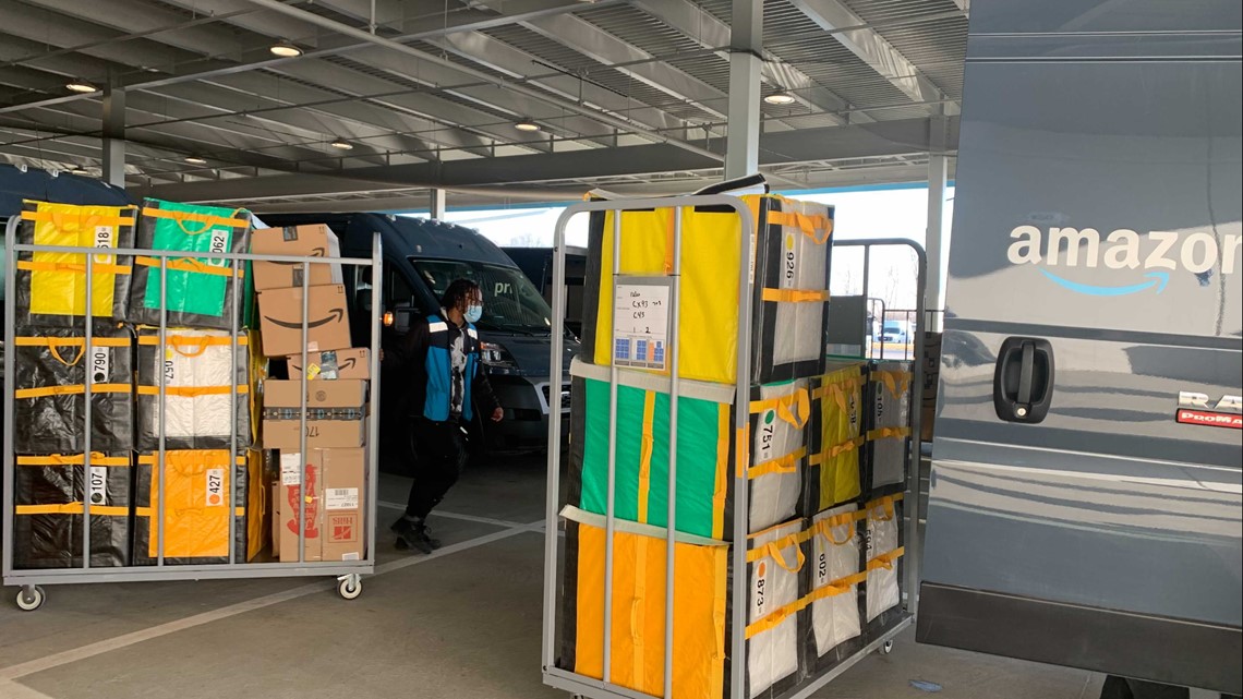
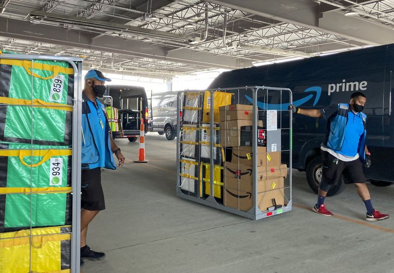
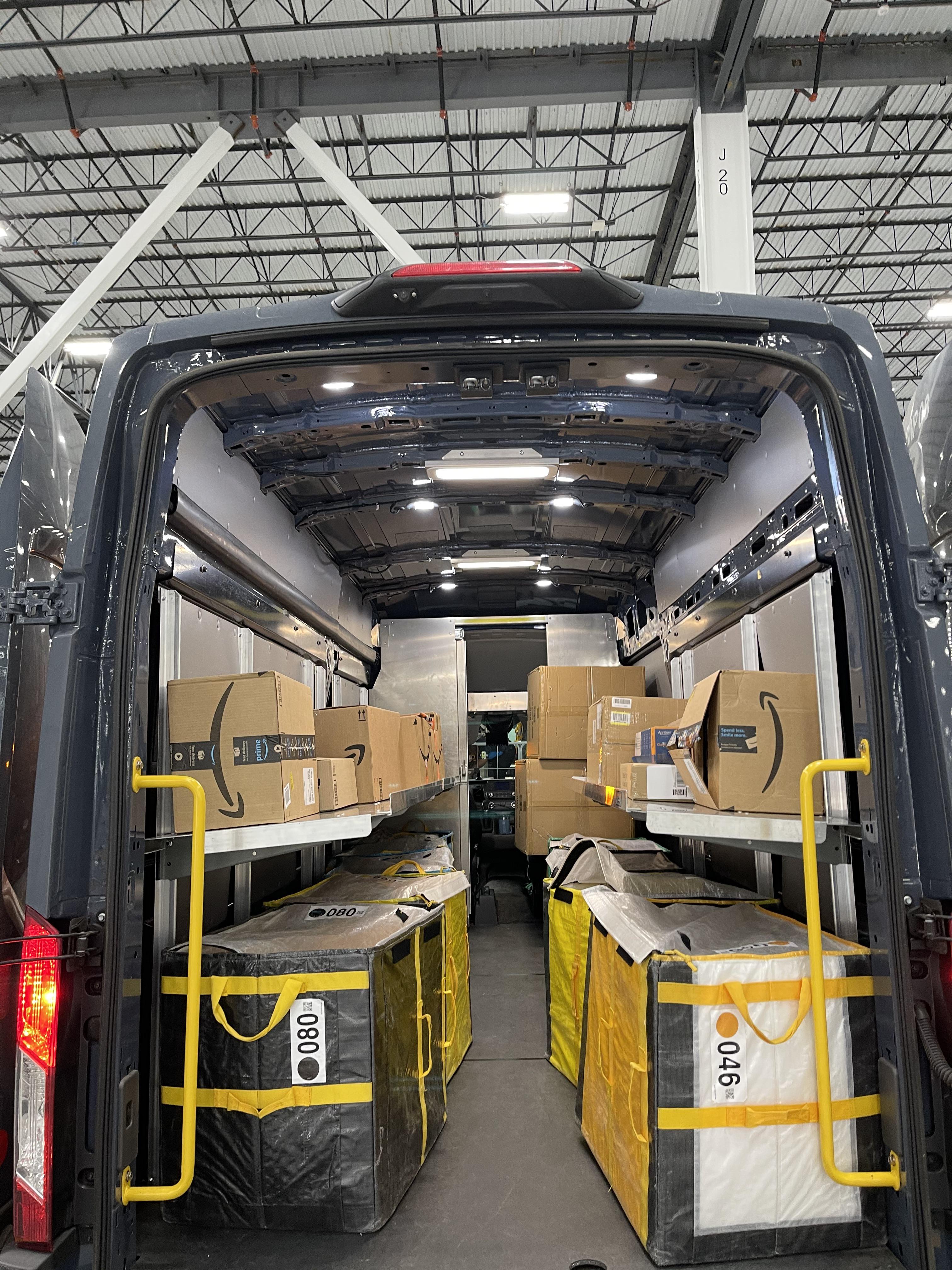
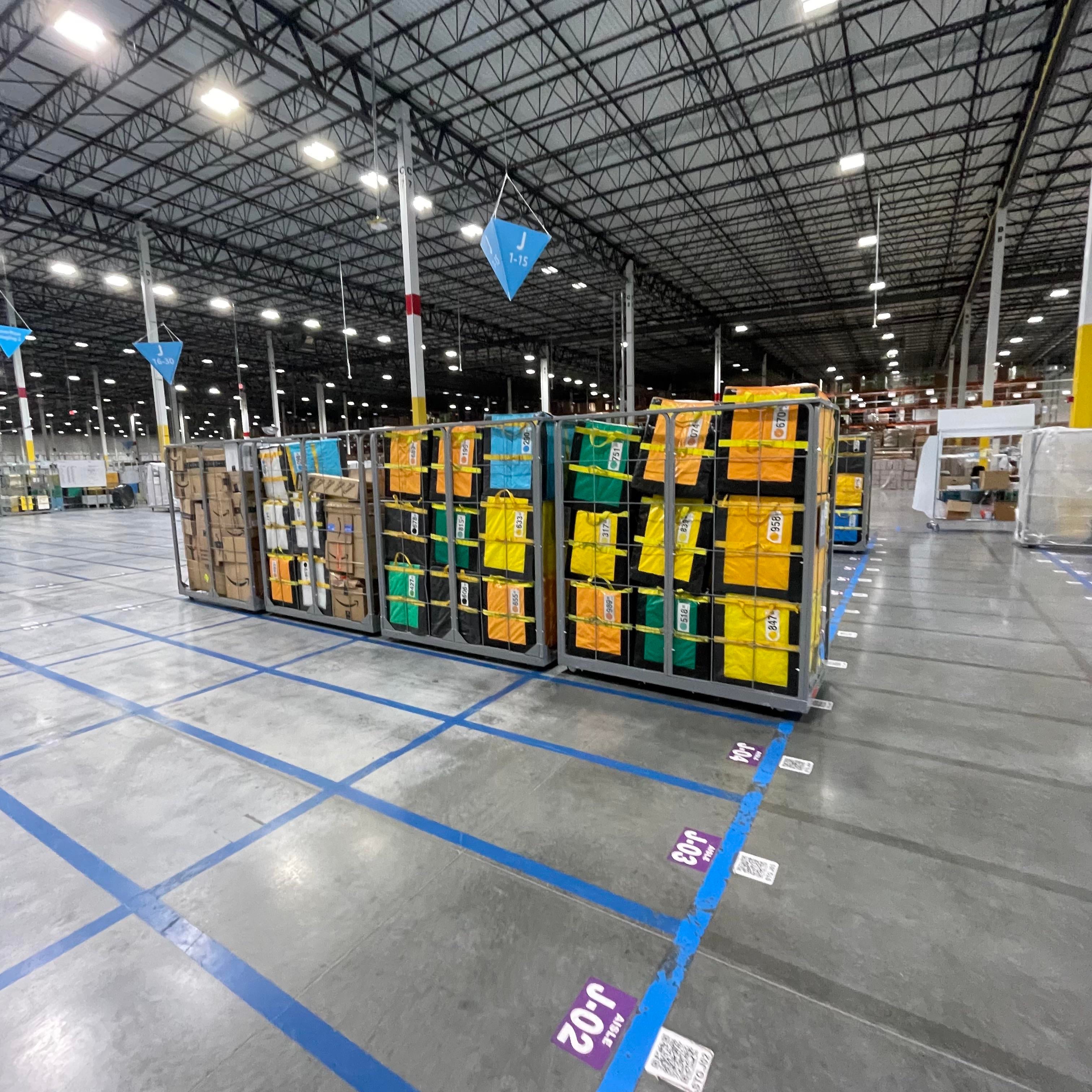
The IDs are used in the van-loading process. The first image below is a photo of a "pick sheet" posted by an Amazon van driver; these sheets are provided to drivers when they arrive at the depot. The "Sort Zone" entries on the sheet have the same form as the IDs on the yellow stickers. Each of the entries on the list points to a collapsible bag, denoted by a color and number. You can see in the second photo that bags stored in the van are indeed labeled with colors and numbers. A reasonable guess then is that bags contain packages having the same zone ID, matching the one on the pick sheet.
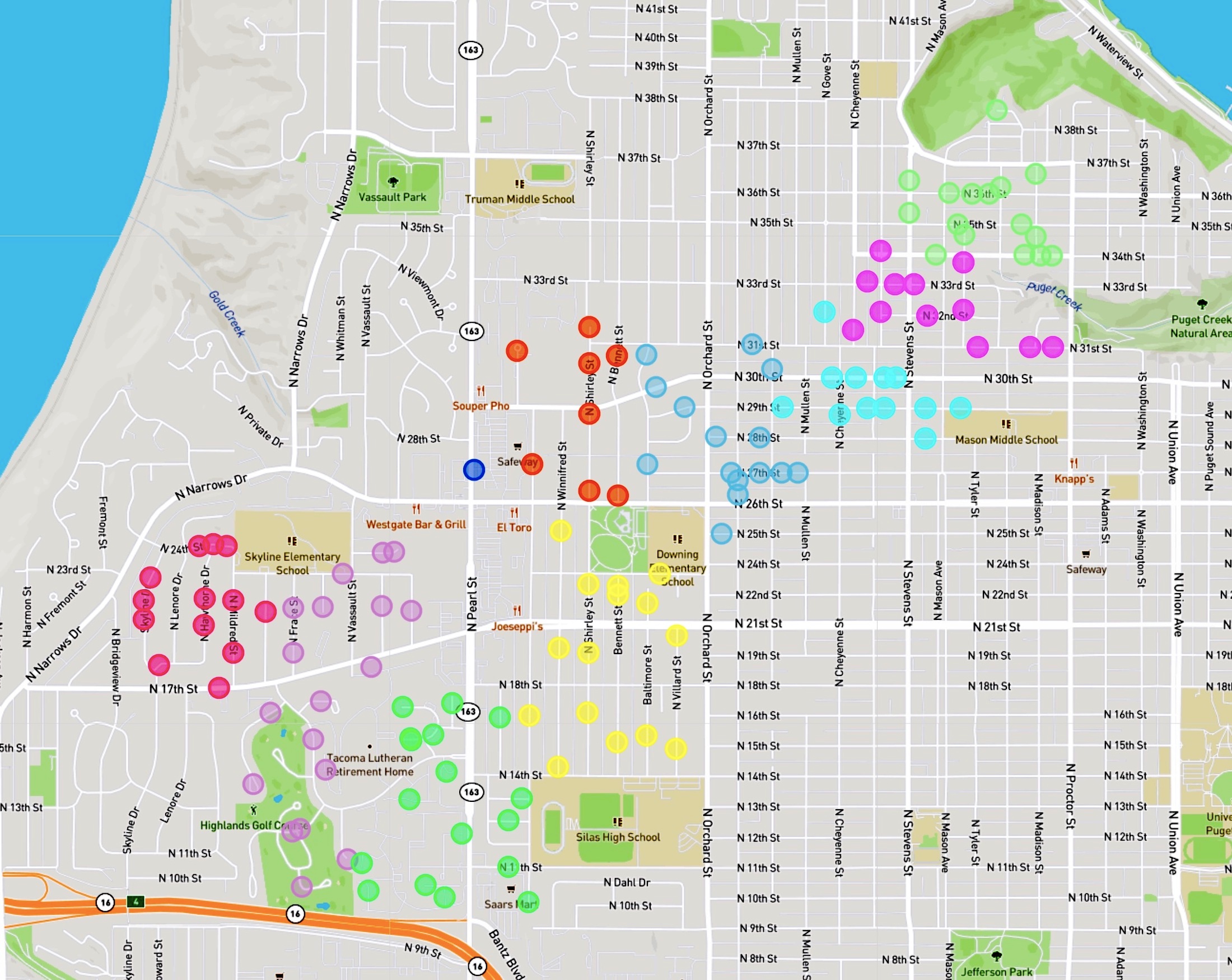
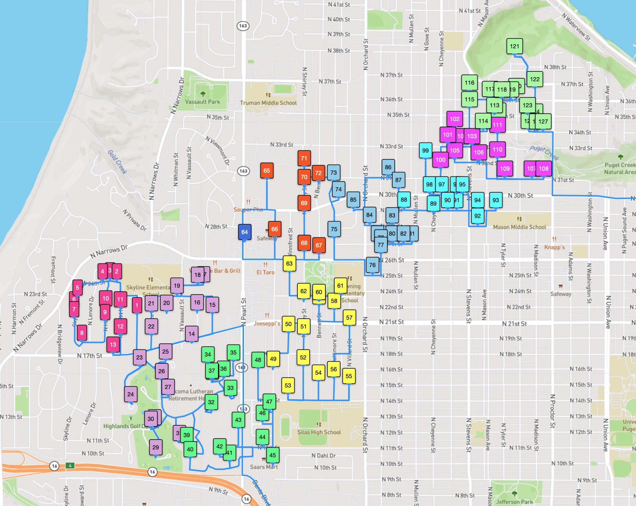
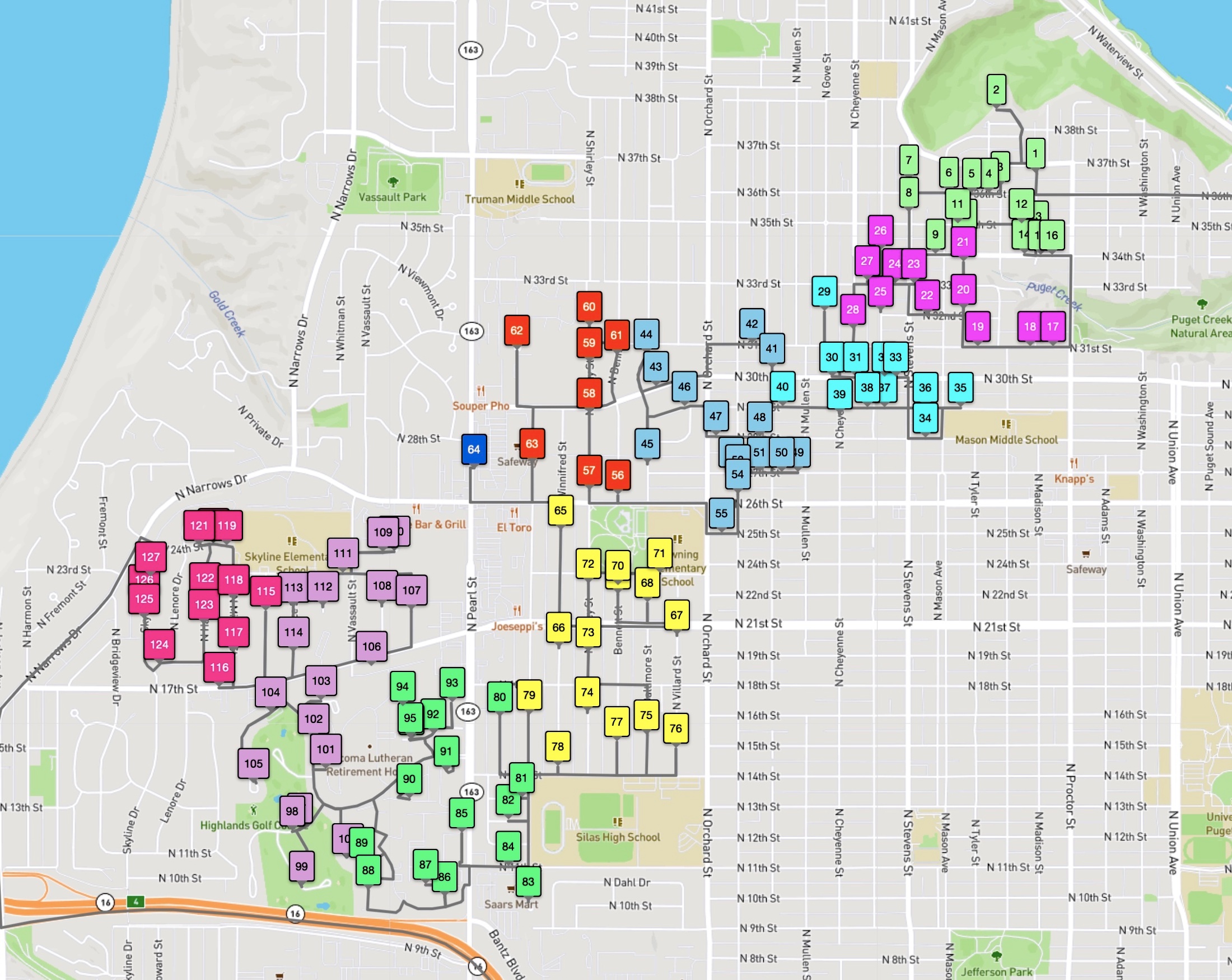
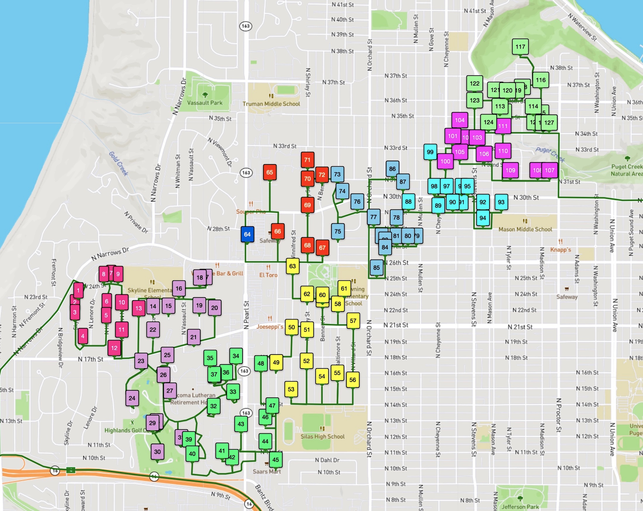
In the following images we have colored the customer stops according to their zone ID. Looking carefully, you can see that the driver visits consecutively all stops having the same ID. Such a routing has an immediate advantage in the organization of the van: the driver empties the bags one-by-one, allowing her/him to collapse the bags and move them out of the way. And steadily working through a bag makes it easy to find packages addressed to the next customer.
The optimal (shortest-possible) tour for this example has many same-colored stops appearing consecutively, but it is quite willing to break this rule to save time in the route. Indeed, the zone ID rule can explain the advantage the optimal tour has over the driver route in the path around the North End Reservoir. The driver is careful to keep the red stops consecutive in the tour order, while the optimal tour moves from a red 48, to a blue 49, and a red 50.
Since drivers tend to keep the zone IDs consecutive in their routes, we can add this condition to our tour-finding algorithms. In the 1,107 examples in the High+Delivered data set, there are an average of 20 distinct zone IDs represented in each route, giving an average of approximately 7 stops per zone. The zones partition the stops in the ATSP instance, where we create a special zone containing only the depot. We use this zone partition to create an instance of the clustered ATSP, where the stops in each zone are required to appear consecutively in any candidate tour. Note that an instance of the clustered ATSP can be transformed to an ATSP by adding a large constant M to the travel time between any pair of stops that do not have matching zone IDs. So we can again apply our traveling-salesman-problem techniques to find optimal solutions to the clustered ATSP instances.
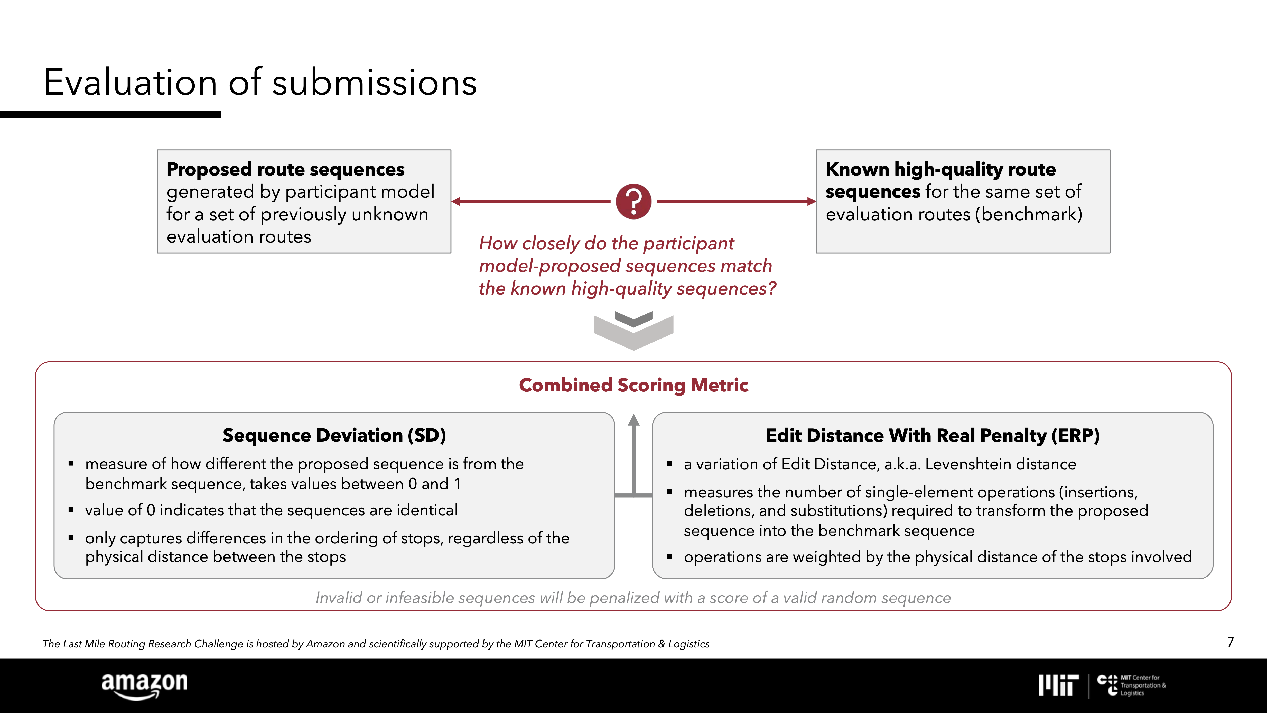
As participants in the Last Mile Routing Research Challenge, our immediate aim is to improve the results our tours obtain on the challenge score metric. Recall that lower scores are better and a perfect match with the driver tour gives a score of 0.0. Over the 1,107 instances in the High+Delivered test set, optimal ATSP tours achieve a score of 0.07030. This is improved to a score of 0.04866 for optimal clustered ATSP tours.
The clustered tours score well, but they are far from perfect matches. The main reason is that an optimal clustered ATSP tour might not follow the zone-to-zone order the driver has chosen. If we knew the driver's zone order, we could gain a big improvement over the clustered ATSP tours, lowering the score to 0.00506.
| Solution Set | Mean Travel Time | Score |
|---|---|---|
| Optimal Tours | 10853.3 | 0.07030 |
| Clustered Tours | 11235.1s | 0.04866 |
| Zone-Ordered Clustered Tours | 11725.1s | 0.00506 |
| Driver Tours | 12250.0s | 0.00000 |
We of course will not be given this order in the scoring phase of the competition. Here is where the training data comes into play. We will examine the data at the zone level, rather than at the house level, looking for patterns in the zone-to-zone choices made by the van drivers. The patterns will be converted into constraints to guide our tour selection algorithm.
The computational results we have presented thus far were obtained with the Concorde TSP solver. Concorde is an exact solver. That is, Concorde finds a TSP tour together with a proof that the tour is shortest possible. This is great for obtaining benchmark results such as those reported in the above table, but for the competition we want better control over the speed of our code (in some of the Amazon cases, Concorde requires 30 minutes or more to prove a solution is optimal) and greater flexibility in allowing us to constrain our tours to match choices likely to be made by drivers.
For this, we adopt a local search approach. The general idea of local search is simple. Starting with any candidate solution, you repeatedly look for small alterations that can lead to a better solution. For the TSP, the common choice for a "small alteration" is to remove a subset of k edges from the candidate tour and reconnect the resulting paths into a new tour by adding k other edges. In a k-opt algorithm, we replace the candidate tour by the new tour (the one we get by reconnecting the paths) if the new tour has shorter length. The simplest version of this (but still very useful in practical applications) is the 2-opt algorithm created by Merrill Flood in the 1950s, where pairs of edges are removed and the resulting two paths are reconnected into a tour.
Our local search code, called LKH-AMZ, is based on the LKH-3 code of Keld Helsgaun. It is designed to give great flexibility in the types of constraints you may want to include in the tour selection, such as the constraint that subsets of stops appear consecutively in the clustered ATSP instances. The "small alterations" used in the code consist of special types of 3-opt and 4-opt exchanges.
In the code, when evaluating a tour T, we assign a penalty to T for any violated constraints. Let penalty(T) denote the sum of the penalties for T and let length(T) denote the length of T. The current candidate tour T is replaced by a new tour T' (where T' is obtained by a 3-opt or 4-opt exchange) if length(T') < length(T) and penalty(T') ≤ penalty(T). That is, we accept a 3-opt or 4-opt exchange if it decreases the length of the tour and does not increase the penalty. A sequence of such exchanges will drive down the length of the candidate tour without increasing the sum of the penalties from violated constraints. Note that we are treating the constraints as "soft", meaning that the tour produced by the algorithm may not necessarily satisfy all constraints, but we aim to have very few violations.
To prevent the code from quickly getting stuck at a poor solution (for example, a short tour having many violated constraints), we run an iterated local search scheme. The process is a bit complex to describe here, so please see our research paper for details.
To give an example of the code's performance when no constraints are present, we ran LKH-AMZ on the ATSP instances obtained from the High+Delivered test collection. In each case we gave LKH-AMZ a time limit of 1 second, running on a 2020 MacBook Air equipped with an M1 processor. These short runs found optimal tours in 1,058 of the 1,107 test instances.
For an example that includes constraints, we ran LKH-AMZ on the 1,107 clustered ATSP instances (handling clusters as constraints, rather than transforming the clustered ATSP to an ATSP). Again using 1 second of running time on the MacBook Air for each example, LKH-AMZ found optimal clustered ATSP tours in 931 instances. Moreover, the LKH-AMZ tours produced a score of 0.04862, improving slightly the 0.04866 score for optimal tours.
Due to the sparsity of the data, houses are not often repeated among the 6,112 training routes. But zone IDs are frequently reused in routes created on different days. We therefore used a simple procedure to see if we could "learn" patterns from the training data, suggesting how driver tours move between zones.
The target of our procedure is to construct precedence constraints, requiring that a particular zone X must be visited before another zone Y. We do this, for a route R, by finding in the training data a route Q that covers many of the same zone IDs as R. We then create a directed graph representation for Q, where the nodes in the graph correspond to the zones covered in Q and a directed edge (A, B) indicates that in route Q the zone A is visited immediately before the zone B. An analysis of this graph for route Q allows us to extract precedence constraints that we impose on the tour we want to construct for route R.
Zone precedence constraints are easily handled in LKH-AMZ. Indeed, at each iteration we make a pass through the current tour T and for each zone X compute the value visit(X) giving the position of the first occurrence of X in T. We then run through the listed precedence constraints (X, Y), adding a constant value ppred to penalty(T) if visit(X) > visit(Y).
Adding precedence constraints to the clustered ATSP models produces a score of 0.03322 on the High+Delivered test instances. This result is for tours produced by LKH-AMZ with a 1 second time limit per route, running on the MacBook Air.
So far, so good. On May 15, 2021, our code was top ranked in a preliminary scoring round, where 600 test instances hidden from the participants were used to evaluate the codes.
But with over a month to go in the competition, we knew we needed to improve our results, driving the score closer to 0.0.
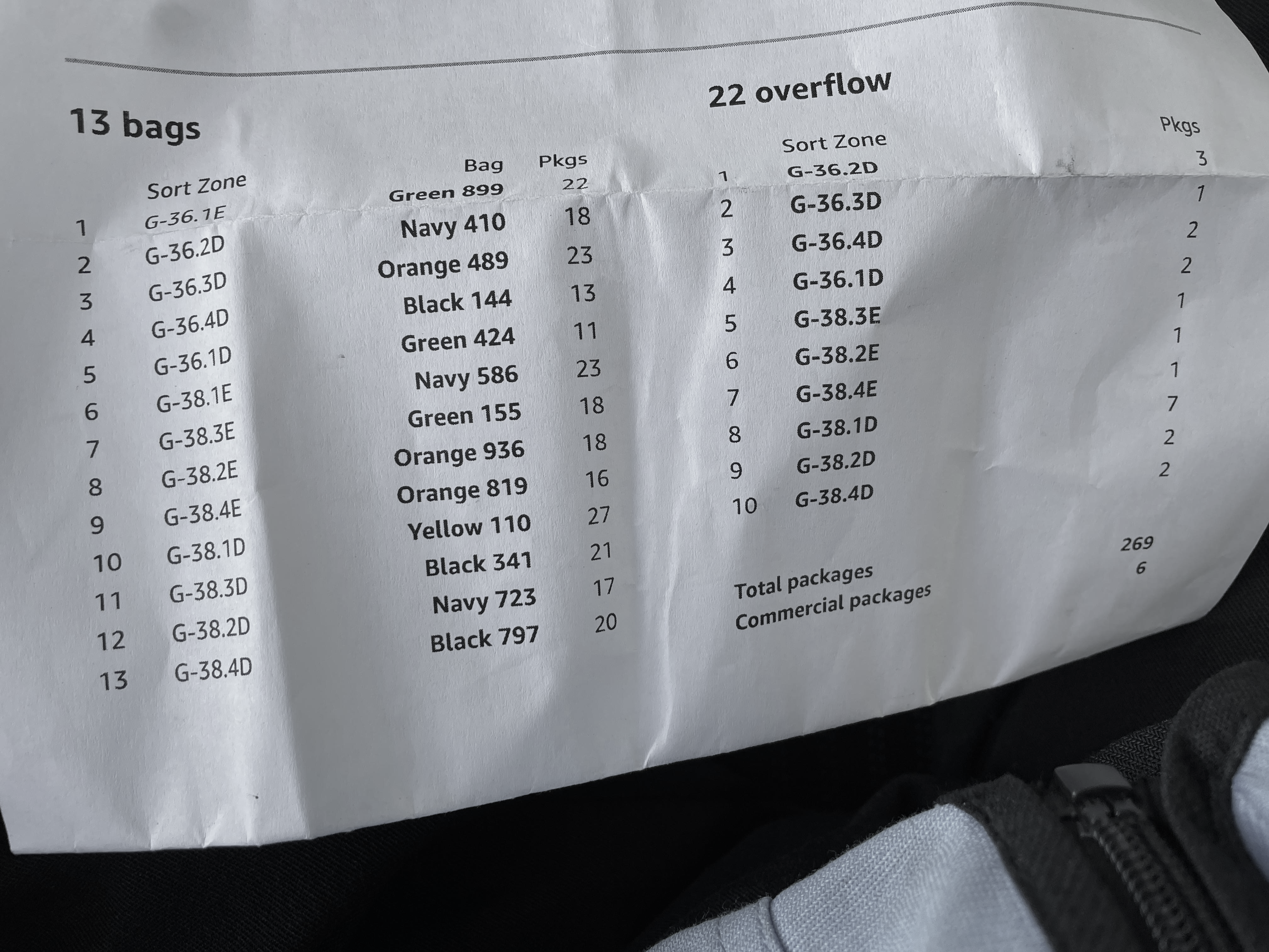
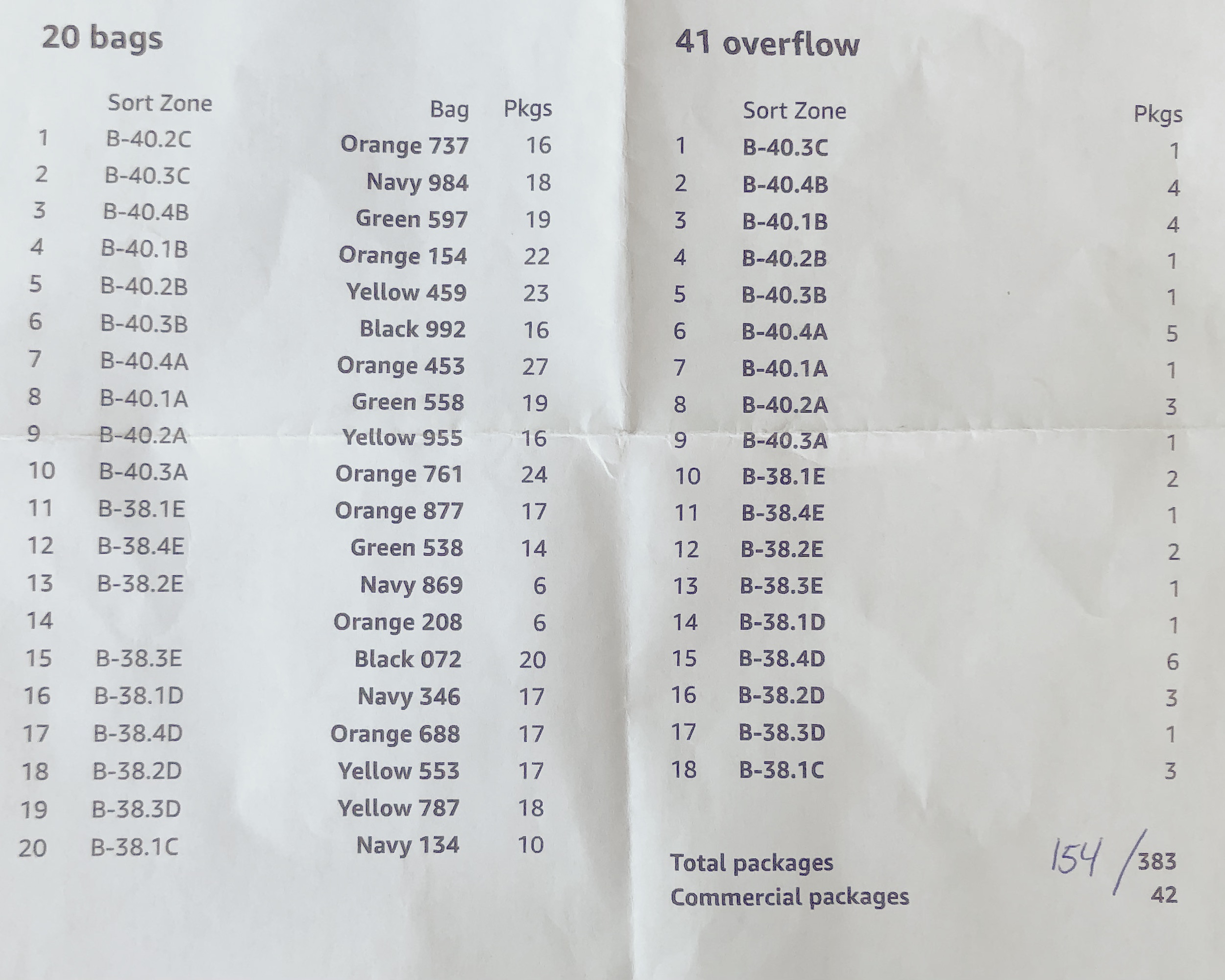
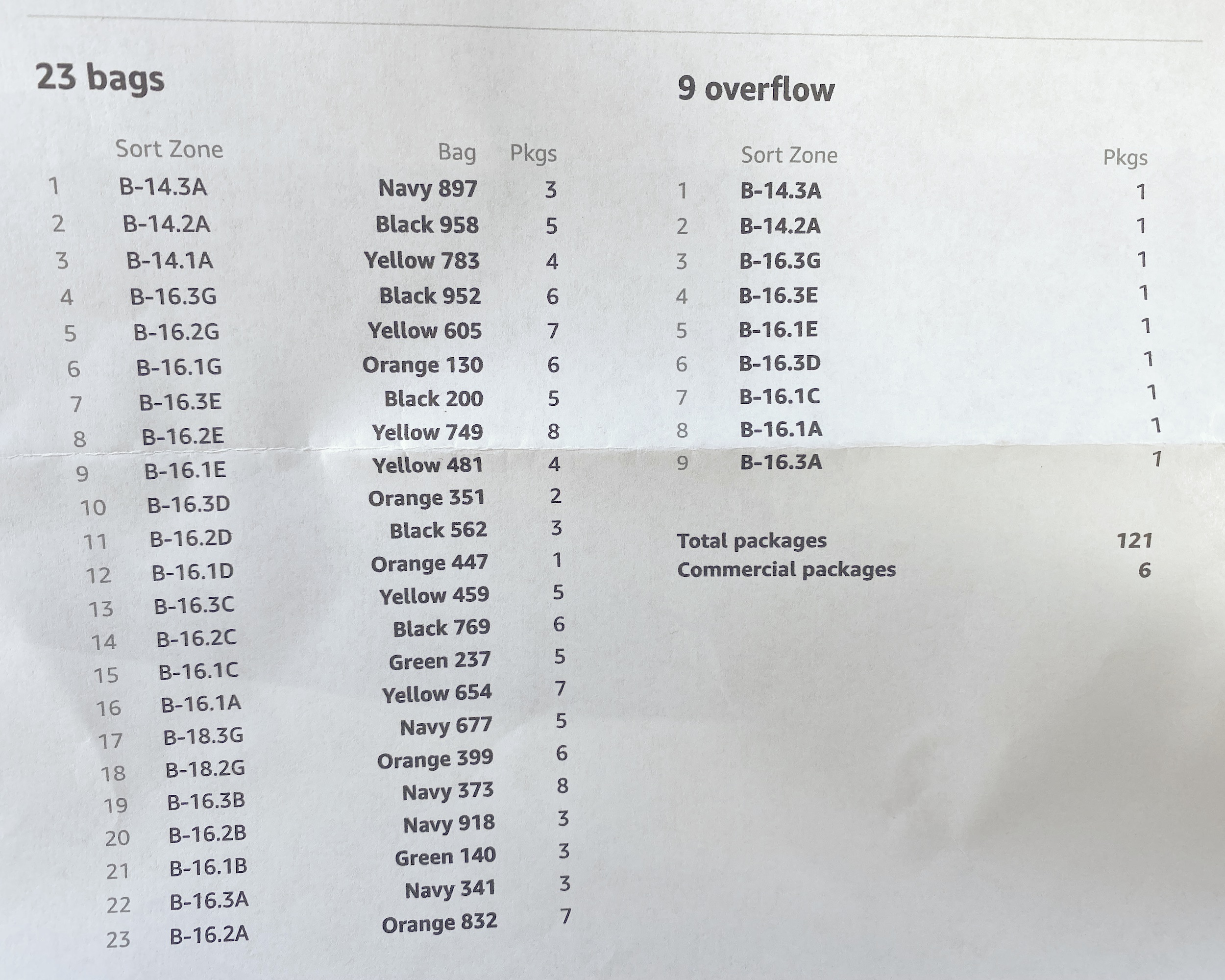
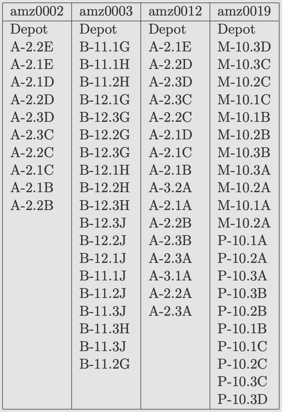
An easy idea for this arose when we examined a sample of the zone orders from the High+Delivered instances. In the image below we list these orders for the first 4 instances in the High+Delivered data set.
There are clear patterns in the zone orders, such as the groupings containing IDs ending in "E", "D", "C", and "B" in the amz0002 instance. These patterns are also evident in pick sheets posted by Amazon drivers. And, looking at the third photo below, one can guess that patterns may influence how bags are loaded in the depot staging area, where carts are made ready for pick up by drivers.
Using a short code to analyze the patterns, we exploit zone IDs to create super clusters (that is, clusters of zone clusters), super-super clusters (that is, clusters of super clusters), and super-cluster-precedence constraints. Adding these to our previous models improved the score to 0.01993 on the High+Delivered instances, again using 1 second runs of LKH-AMZ on the MacBook Air.
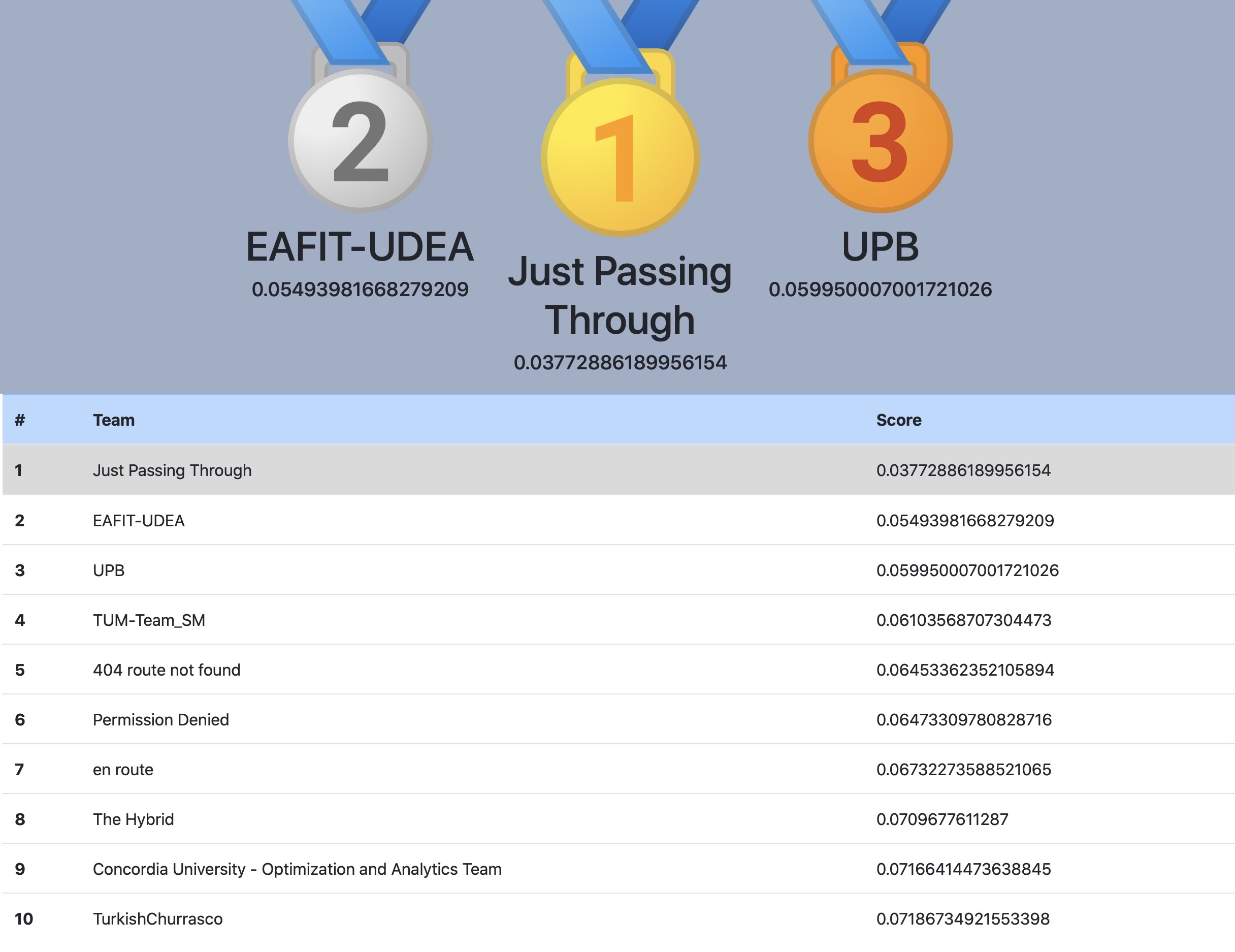
After several additional tweaks, we submitted a final code to the competition on June 18, 2021. Our Just Passing Through team was announced as the winner of the $100,000 top prize on July 30, 2021.
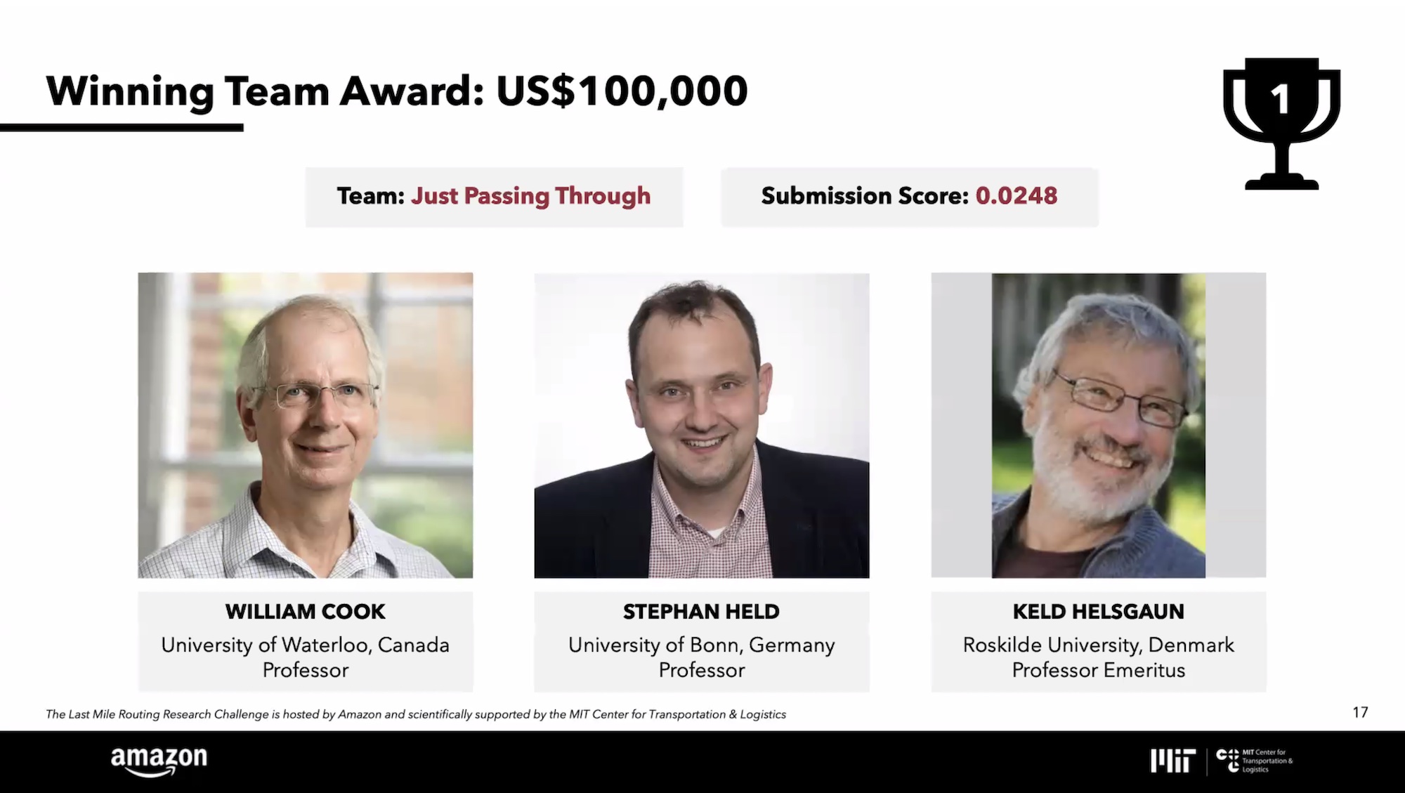
The solution approach falls under the general umbrella of traditional optimization-driven operations research, and thus does not match well the Last Mile Routing Research Challenge call for work "leveraging artificial intelligence, machine learning, deep learning, computer vision, and other non-conventional methods." The competition score for our Just Passing Through team was substantially better than scores for all other competitors (and the second and third place teams also adopted what can be viewed as traditional optimization methods).
At this point, it appears that mathematical optimization is superior to machine-leaning techniques for producing high-quality tours. Nonetheless, the nice research by many of the teams in the Last Mile Routing Research Challenge points to an important role for machine learning in this context: given much larger data sets of training routes, sophisticated learning approaches could reveal important patterns in the historical data. Such patterns could be worked into constraints that are expected (or desired) to hold in practical routing solutions. These then could be fed into a constrained local-search method such as we adopt in LKH-AMZ. Our code is designed to be very flexible, allowing the computer implementation to be easily modified to handle new applications.
The source code for LKH-AMZ (written in the C programming language) is available on the JPT-AMZ GitHub page. The code links only the standard C library, making it easily portable to many computing platforms. It is distributed under the MIT License, allowing for use in both commercial and non-commercial applications.
Please see our research paper Constrained Local Search for Last-Mile Routing for a detailed description of the algorithm behind LKH-AMZ and how we used the code in the competition.
Finally, let me remark that by sponsoring the Last Mile Routing Research Challenge and releasing the huge collection of test data, Amazon has shown great support for the general research community. The traveling salesman problem is clearly important for the efficient operation of their delivery service and it is fantastic that the company has worked to connect with academic researchers.
We thank Amazon, MIT, and the organization team for running an excellent competition.
Photo credits. The three van-packing photos at the top of the page appeared in the web pages of WTHR, The Baltimore Sun, and Amazon. The pick sheets and zone bag photos are from posts on the Amazon DSP Drivers section of reddit.com.