A beauty of the TSP is that it is fundamental in so many applications, from genome mapping through computer-circuit design.
Whenever you have to put objects into a sequence, there may be an example of the TSP waiting to be solved.
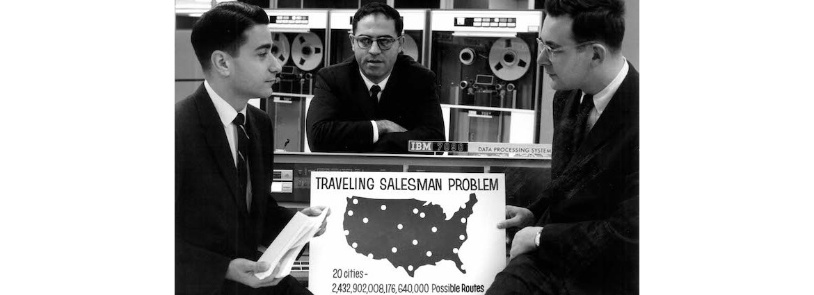
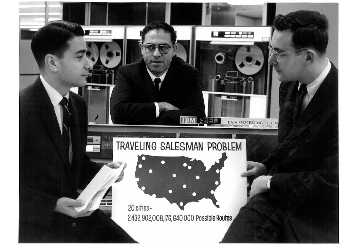
That said, there is no doubt that, when you hear "traveling salesman problem," what comes to mind is a person moving around the country, pulling into city after city along the way.
In fact, this vision for the mathematical problem pre-dates the TSP name.
In the 1930s, the main proponent of the problem was Hassler Whitney, who described the challenge of finding a shortest route to visit one city in each of the USA states.
Here is what Operations Research pioneer Merrill Flood explained in an interview.
Developments that started in the 1930s at Princeton have interesting consequences later. For example, Koopmans first became interested in the "48 States Problem" of Hassler Whitney when he was with me in the Princeton Surveys, as I tried to solve the problem in connection with the work by Bob Singleton and me on school bus routing for the State of West Virginia. I don't know who coined the peppier name 'Traveling Salesman Problem' for Whitney's problem, but that name certainly has caught on, and the problem has turned out to be of very fundamental importance.
Perhaps the first time the TSP name appears in print is in a RAND report by famed mathematician Julia Robinson.
In describing the problem, she writes "One formulation is to find the shortest route for a salesman starting from Washington, visiting all the state capitals and then returning to Washington."
Road travel is definitely what early TSP researchers had in mind.
The California experts
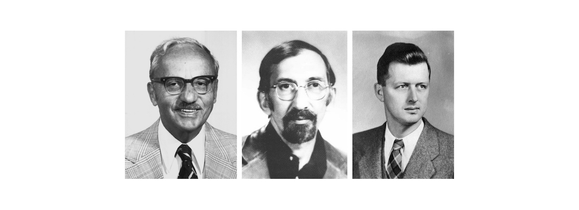
The heroes here are George Dantzig, Ray Fulkerson and Selmer Johnson.
In 1954 they settled Whitney's challenge.
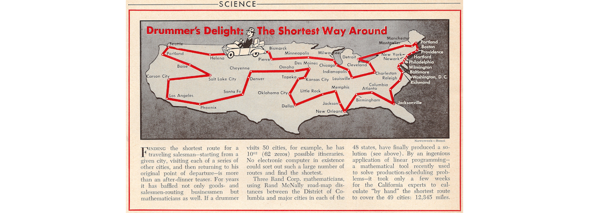
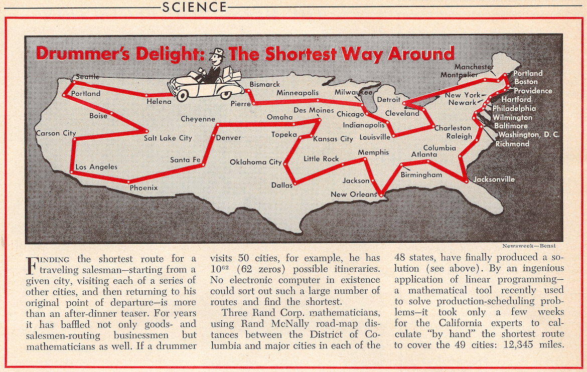
Here is how it was reported in Newsweek.
By an ingenious application of linear programming - a mathematical tool recently used to solve production-scheduling problems - it took only a few weeks for the California experts to calculate by hand the shortest route to cover the 49 cities.
The abstract to their RAND Corporation research paper is beautifully succinct: "It is shown that a certain tour of 49 cities, one in each of the 48 states and Washington, D. C. has the shortest road distance."
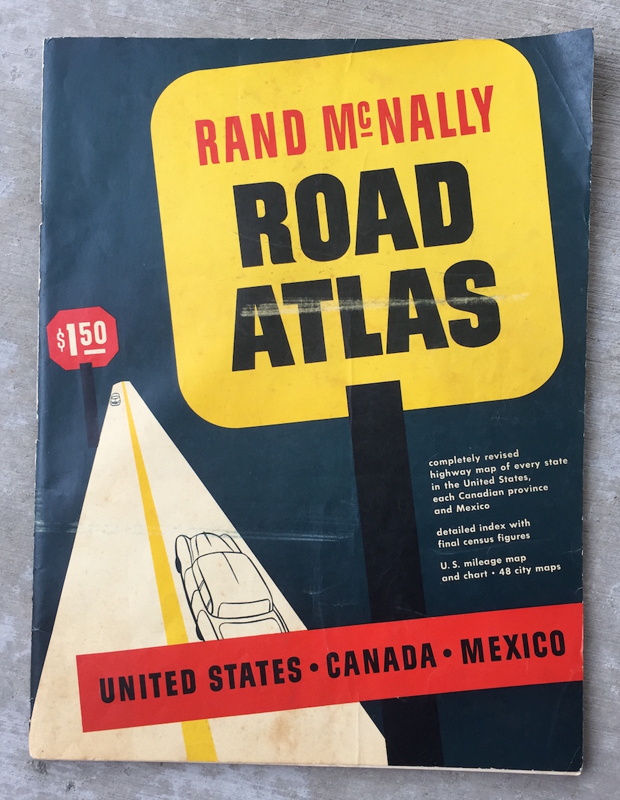
Regarding the choice of the city in each state, the team writes "The reason for picking this particular set was that most of the road distances between them were easy to get from a Rand McNally atlas."
It is perhaps a sacrilege to say this, since all computational TSP work stands on the broad shoulders of Dantzig's team, but at the start of their project they made a change to the Rand McNally road data that likely made the problem technically much easier to handle.
I was able to buy a 1954 Rand McNally Road Atlas on eBay.
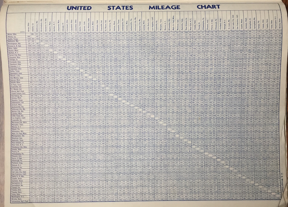
It contains a mileage table for 60 cities, with partial information for 15 others.
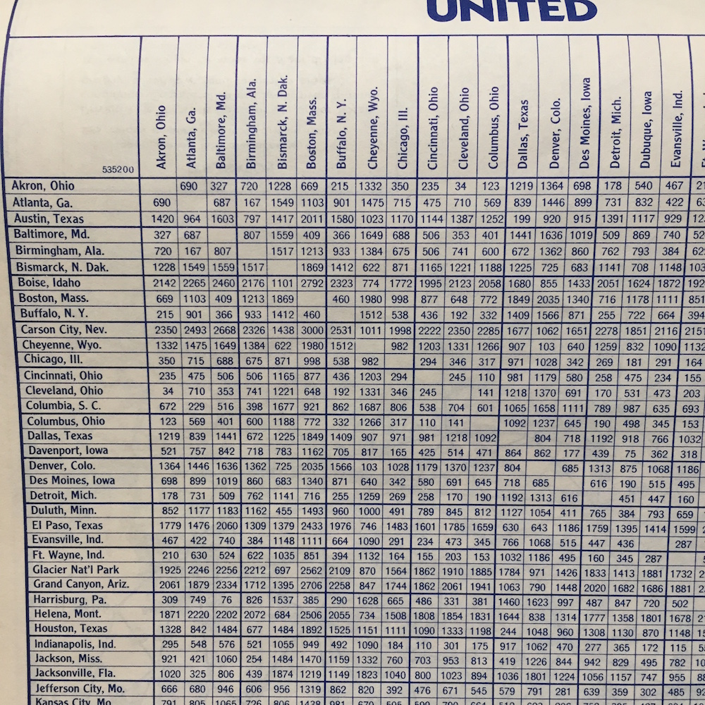
In a close-up view you can read the point-to-point driving distances.
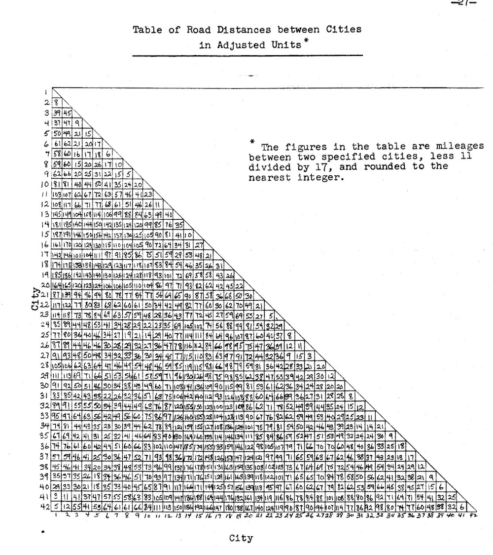
Now compare this with the distance matrix from the original paper by Dantzig et al.
What you see is that the numbers in the paper are much smaller.
Dantzig's team did not hide this transformation.
Notice that their heading is "Table of Road Distances between Cities in Adjusted Units."
In their paper they describe the precise transformation: distance d is replaced by the nearest integer to (d - 11)/17.
They write "This particular transformation was chosen to make the d in the original table less than 256 which would permit compact storage of the distance table in binary representation; however, no use was made of this."
Their overall strategy did not depend on the small numbers, but it certainly made their calculations easier to carry out by hand.
So perhaps we should use an asterisk when we call their result a road TSP.
It remains, nonetheless, the greatest computational result in the history of the problem and their test instance was obviously motivated by road travel.
Numbers pouring out
In his Turing Award lecture, the great computer scientist Richard Karp made the following remark.
I don't think any of my theoretical results have provided as great a thrill as the sight of the numbers pouring out of the computer on the night Held and I first tested our bounding method.
Those pouring numbers in 1970 included the solution of a 57-city TSP, finally breaking the record set by Dantzig's team 16 years earlier.
There is a story behind the TSP example solved by Karp and his IBM colleague Michael Held.
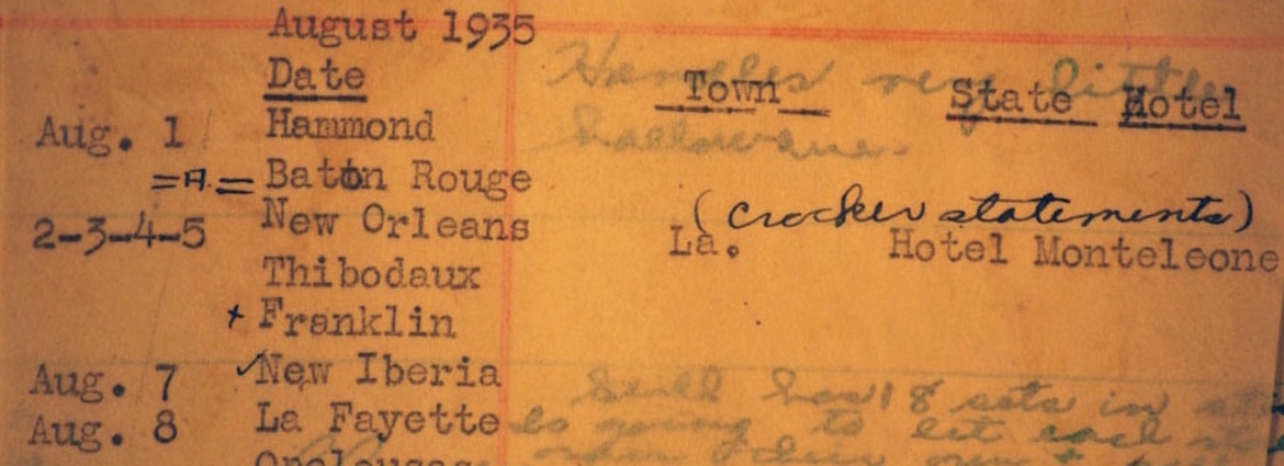
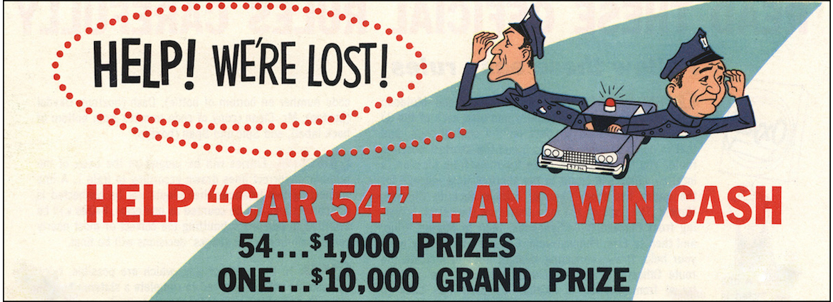
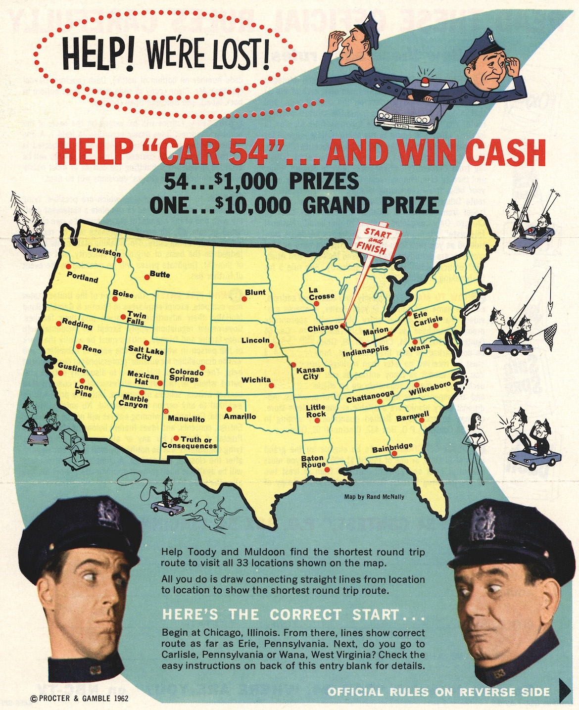
In 1962, Procter & Gamble ran a contest asking for the shortest tour through 33 cities in the US, using Rand McNally road distances.
At this point, the TSP was already a well-studied model in applied mathematics and operations research, but the $10,000 prize certainly brought added attention to the problem of finding good tours.
Among the new TSP devotees were researchers Robert Karg and Gerald Thompson.
In work at the Carnegie Institute of Technology, they designed a practical tour-finding method that could be implemented on an electronic computer.
The results of their computer code did not come with guarantees to be shortest possible, but their 33-city solution was good enough to come in tied for first place in the Procter & Gamble contest.
With their Bendix G-20 computer to do the heavy lifting, Karg and Thompson thought, why not tackle some larger problems?
So they used their atlas to create a new challenge instance with 57 cities.
I don't have a 1962 Rand McNally atlas, but I note that Karg and Thompson's list includes 57 of the 60 cities from the 1954 atlas.
Two of the missing entries are Montreal and Mexico City.
Fair enough, in keeping within the US borders.
The third missing city is Dubuque, Iowa.
This perhaps came from a quirk in Rand McNally's typesetting, where Dubuque appears in the horizontal list by not the vertical list.
You can find the problem data here in TSPLIB format.
Karg and Thompson used the point-to-point mileage reported by Rand McNally, so no asterisk this time.
And hats off to them for using the full available data set (except for the oddly typeset Dubuque).
Although Karg and Thompson did not know it at the time, the 33-city tour reported in their 1964 research paper was in fact optimal.
This was not the case for the 57-city problem: their best tour had length 12,985 miles, but they mentioned that another research group found a tour that was 30 miles shorter, but still with no guarantee of optimality.
Held and Karp's big night of computing in 1970 showed that there were no further miles to be shaved from the tour, they proved that 12,955 was indeed the shortest-possible mileage.
Man + Machine
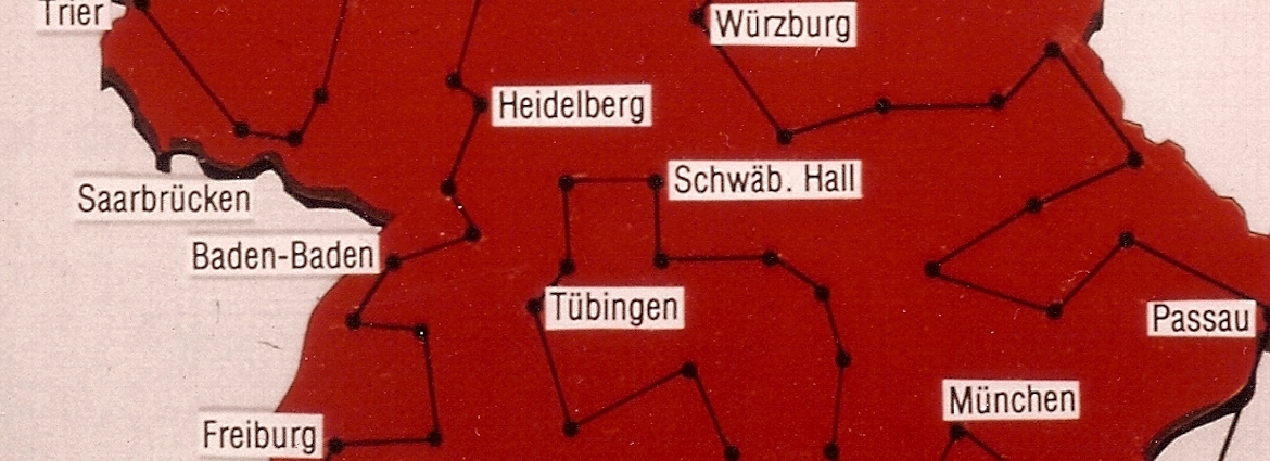
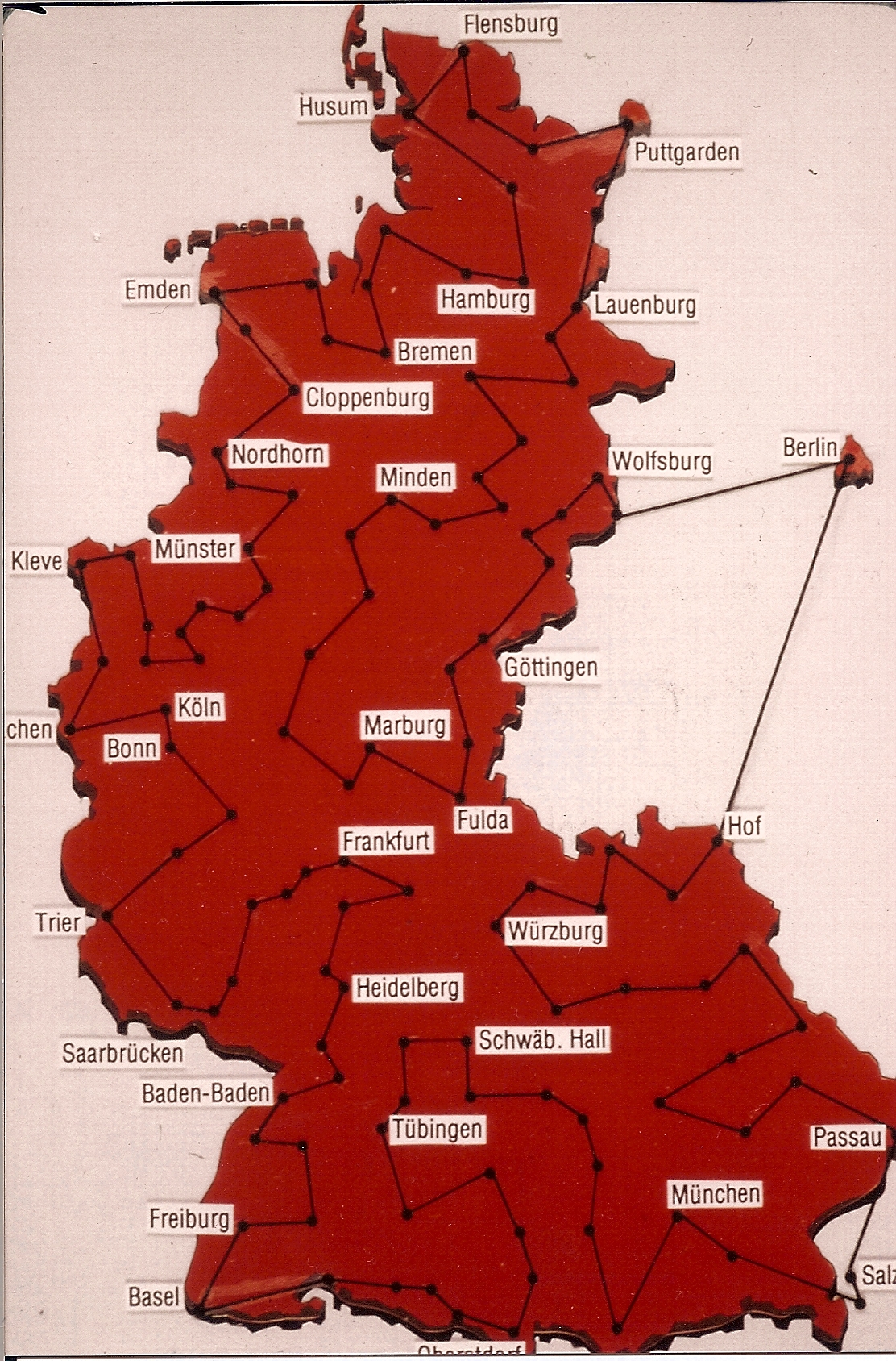
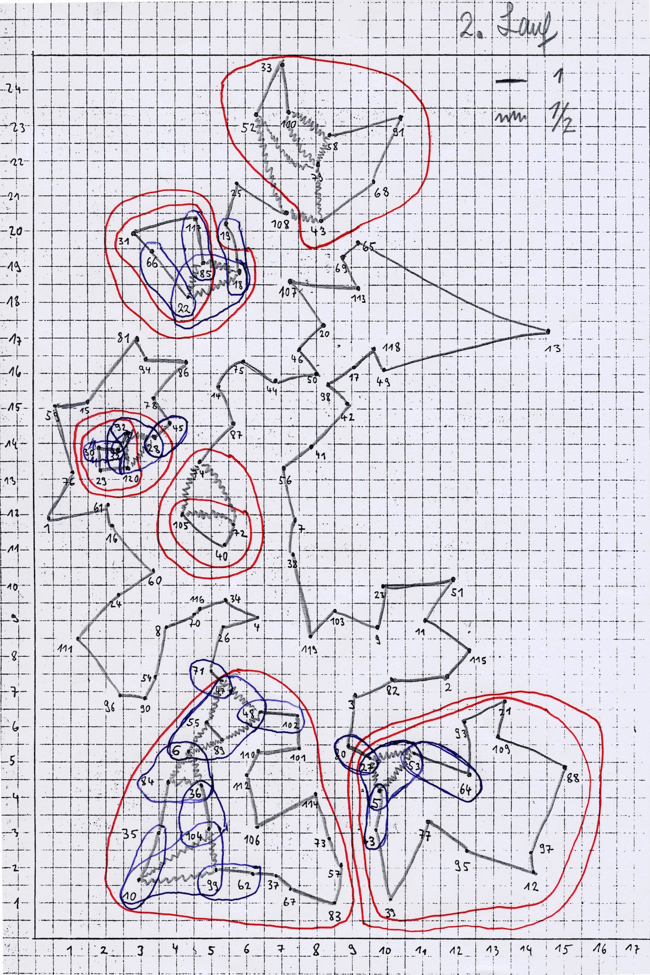
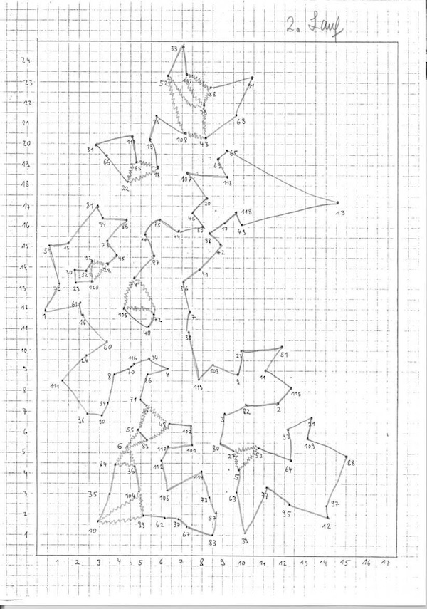
Martin Groetschel, the current President of the Berlin-Brandenburg Academy of Sciences and Humanities, pushed the road-TSP record to 120 cities as part of his PhD work in 1977.
Definitely no asterisk here.
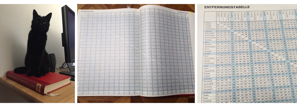
His challenge problem used the full distance-table in the 1967/68 edition of the Deutscher General Atlas, with point-to-point distances measured in kilometers.
Again, a tip of the hat to him for taking all of the available data.
In setting their TSP record, Dantzig's team adopted by-hand computations, while Held and Karp used an IBM computer.
Groetschel?
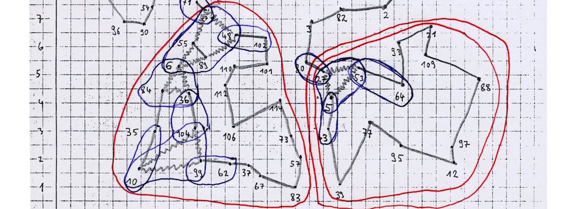
He used both.
A large part of his computation was carried out by hand, taking a drawing of the current linear-programming solution and finding cutting planes to add.
The LP models themselves were solved on a big-iron machine, an IBM 370/168 at the University of Bonn.
Groetschel concludes his research paper with the line "Readers interested in trying their TSP-code or -heuristic on the 120-city problem solved in this paper can obtain a card deck with the road distances between the above listed cities from the author."
No need to trouble Dr. Groetschel for the punched cards, here is the data set in TSPLIB format.
TSP Pursuit
If you happen to be interested in the history of the TSP, may I humbly suggest you have a look at the Princeton University Press book In Pursuit of the Traveling Salesman: Mathematics at the Limits of Computation.
It is a small volume, but it gives a detailed look at the history of the problem, its applications, and the techniques that have been used to tackle it.
