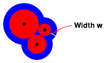
The most natural way to describe a TSP tour is to give a list of the cities in the order they should be visited, that is, an itinerary for the trip. To construct lower bounds, however, it is often useful to consider an alternative tour description where we list the roads that are used by the tour. In this context, by a "road" we mean the direct trip between a pair of cities in the TSP.

Consider the 6-city TSP drawn below. A tour in this instance corresponds to a selection of 6 of the 15 possible roads between the points.

To describe the selected roads, it is again useful to have some standard mathematical notation. We will name the cities 1, 2, 3, ... , n, and for two cities i and j we let x(i,j) indicate whether or not we choose the road between i and j in our tour, that is, if we use the i-to-j road then we set x(i,j) = 1 and if we do not use the i-to-j road then we set x(i,j) = 0.

Now since the i-to-j road is the same as the j-to-i road, we only need to specify the value of x(i,j) for those pairs of cities where i is less than j. In this formulation, for a TSP with n cities we have n(n-1)/2 variables x(i,j) that must be determined.

To calculate the length of a tour we need to add up the distances dist(i,j) for each road that we use. The variables x(i,j) give us a handy way of doing this, since the expression

dist(i,j)x(i,j),

that is, dist(i,j) multiplied by x(i,j), is equal to d(i,j) if we use the road and 0 if do not use the road.

Therefore, we get a formula for the length of a tour by adding up the expressions d(i,j)x(i,j) for all pairs of cities i, j.

Tour Length = dist(1,2)x(1,2) + dist(1,3)x(1,3) + ... + dist(n-1,n)x(n-1,n)

Notice that this formula is a weighted sum of the variables and so it can be used as the objective function for a linear programming (LP) problem (where the x(i,j) variables can possibly take on fractional values, not just 0 and 1). To use this observation to obtain TSP lower bounds, we just need to build some constraints on the variables that capture some of the properties of tours.

To start off, notice that for each city i we must select two of the roads that start or end at i (since we need to arrive at city i and then leave again). We know, therefore, that if we add up the n-1 variables that correspond to these roads we must get the sum of 2. We use this to get the following simple LP relaxation of the TSP known as the fractional 2-matching LP.

Minimize dist(1,2)x(1,2) + dist(1,3)x(1,3) + ... + dist(4,5)x(4,5)

Subject To

x(1,2) + x(1,3) + x(1,4) + x(1,5) >= 2

x(1,2) + x(2,3) + x(2,4) + x(2,5) >= 2

x(1,3) + x(2,3) + x(3,4) + x(3,5) >= 2

x(1,4) + x(2,4) + x(3,4) + x(4,5) >= 2

x(1,5) + x(2,5) + x(3,5) + x(4,5) >= 2

x(1,2) >= 0, x(1,3) >= 0, ... , x(4,5) >= 0

Each tour (or more precisely, the corresponding assignments of 0's and 1's to the variables) satisfies all constraints of the LP and is therefore a candidate LP solution. Of course, there are many LP solutions (including fractional ones) that are not tours and so we would not often be able to solve the TSP by applying the simplex method to the LP. If we are lucky, however, and the optimal solution to the LP is indeed a tour, then we know that this tour is also an optimal solution to the TSP (since the LP objective minimizes the tour length and every tour is a candidate LP solution).

Even in the more common case when the optimal LP solution does not correspond to a tour, the optimal value of the objective function is a lower bound for the TSP since no tour can give the objective a smaller value.

The question of the quality of this lower bound brings us back to the control-zone bound for the TSP. Given a non-overlapping collection of disks, twice the sum of their radii is also a lower bound for the fractional 2-matching LP! Moreover, the optimal objective value of the LP is equal to the value of best bound that can be obtained with control zones!

The first of these two remarkable facts is easy to see by examining the form of the LP constraints (the sum of the road variables crossing each disk is at least 2). The second fact, that the two lower bounds are equal, is not so easy to see, but it follows from an intimate relationship between the control-zone LP and the fractional 2-matching LP known as LP duality.

A full discussion of LP duality would take us too far astray, but we point out the important fact known as the Weak Duality Theorem that any solution to the dual LP gives a bound on the objective value of the LP itself. This is crucial to the success of LP methods for the TSP since it means that we do not always need to solve the LP exactly to get a lower bound, we just need to find a good solution to the dual LP. We comment further on this point in the Accuracy of Computations page.

Now it is fairly easy to see how we can improve the lower bound we get from the fractional 2-matching (and therefore the bound from control-zones): we just need to build additional constraints that are satisfied by all tours. Adding such constraints to the LP will cut down on the number of candidate LP solutions, potentially raising the optimal objective value of the LP and therefore raising the TSP lower bound.

The first two steps are to note that we can change the ">= 2" constraints to "= 2" (since a tour picks exactly two roads meeting each city) and that we can add the constraint that each x(i,j) be at most 1 (after all, every tour will be either 0 or 1, so there is no need to consider LP solutions that assign values larger than 1 to the variables).

Minimize dist(1,2)x(1,2) + dist(1,3)x(1,3) + ... + dist(4,5)x(4,5)

Subject To

x(1,2) + x(1,3) + x(1,4) + x(1,5) = 2

x(1,2) + x(2,3) + x(2,4) + x(2,5) = 2

x(1,3) + x(2,3) + x(3,4) + x(3,5) = 2

x(1,4) + x(2,4) + x(3,4) + x(4,5) = 2

x(1,5) + x(2,5) + x(3,5) + x(4,5) = 2

x(1,2) >= 0, x(1,3) >= 0, ... , x(4,5) >= 0

x(1,2) <= 1, x(1,3) <= 1, ... , x(4,5) <= 1

These improved constraints are often called the degree equations and the relaxation is referred to as the fractional 2-factor LP.

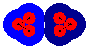
The new relaxation improves the lower bound in many examples, but it does not help in the case given above consisting of the two triangles separated by a gap, since the triangles are also a solution to the fractional 2-factor problem. The next step is to take the bull by the horns and forbid such subtours in our solutions.

To this end, we know that any tour will contain at least two roads going between the two clusters. We can therefore add a constraint that states that the sum of the corresponding variables must be at least two.

More generally, let S be any collection of cities having at least 2 and at most n-1 members (that is, S cannot be the entire set of cities in the TSP) and let T denote the remaining cities. To forbid the subtour through the cities S, we can add condition that the sum of the variables corresponding to roads from S to T must be at least 2.

Quite appropriately, this is called the subtour-elimination constraint for the cities S. The LP we get by adding all such constraints is called the subtour relaxation of the TSP.

The quality of the lower bound we obtain by solving the subtour relaxation is much better than what we get from the fractional 2-factor LP, but notice that it comes at a price --- the number of constraints we now have is far too great to be able to give directly to an LP solver. This difficulty is handled in an elegant manner by Dantzig, Fulkerson, and Johnson, and it just the tip of the cutting-plane-method iceberg that we begin to discuss in the Cutting Planes page.

Let us close our current discussion by describing how Juenger and Pulleyblank complement their control zone idea with an analogue of subtour- elimination constraints. The idea is as follows. Given a collection S of some (but not all) cities, we can draw a region separating the cities in S from those not in S. Now since any tour must visit the collection S, we can add twice the width of the geometric region to our lower bound.

Juenger and Pulleyblank call these geometric regions moats. In terms of linear programming, moats correspond to the dual variables for the subtour-elimination constraints.

For geometric instances, the moat analogy makes it clear why subtour-elimination constraints greatly improve the value of the lower bound -- they allow us to close the gaps that control zones alone could not touch. This is illustrated in the next figure, where we use two moats (one would have been enough) to close the gap in the example given earlier.

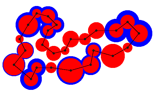
A pretty example of a packing of TSP control zones and moats is given below. Note that lower bound provided by the zones and moats proves that the indicated tour is optimal

As you can see in the figure, although there are very many possibilities for choosing sets of cities, it is sometimes the case that we don't need many different moats to get a good lower bound. It is this observation that motivates Dantzig, Fulkerson, and Johnson's approach to efficiently computing lower bounds for the TSP, as we describe in the Cutting Planes page.