
|
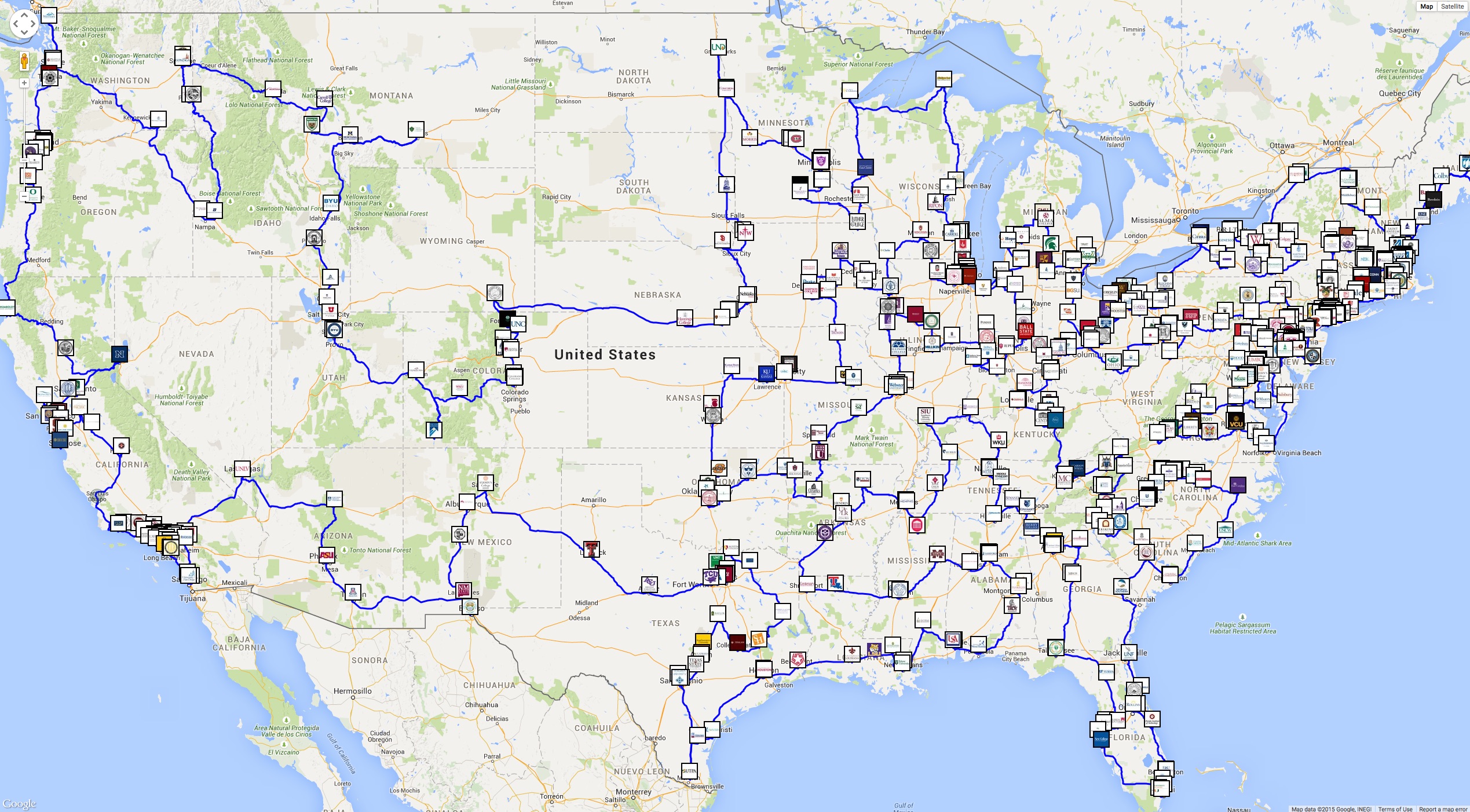
| Portion of optimal college tour. Click for a full image. For an interactive version Click Here. |
Each year, tens of thousands of high-school students and their parents pack up the family car and head out on the road, looking for a chance to visit as many colleges as they can squeeze into their vacation plan. Trips can take several weeks, but time invariably runs out with many great campuses still waiting to be seen. So why not visit them all!
For the most gung-ho of aspiring students, I computed the shortest road trip to visit all 647 campuses on Forbes' list of America's Top Colleges.
|
|
| Portion of optimal college tour. Click for a full image. For an interactive version Click Here. |
You'll need a good-sized budget for gasoline: the optimal tour covers 29,297 miles. To be precise, with the travel distances we have from Google Maps, the tour takes 47,149,705 meters. And this is the best possible. If you don't believe me, here are the distances I used. I offer a $1,000 prize to the first person who finds a shorter tour with this distance table.
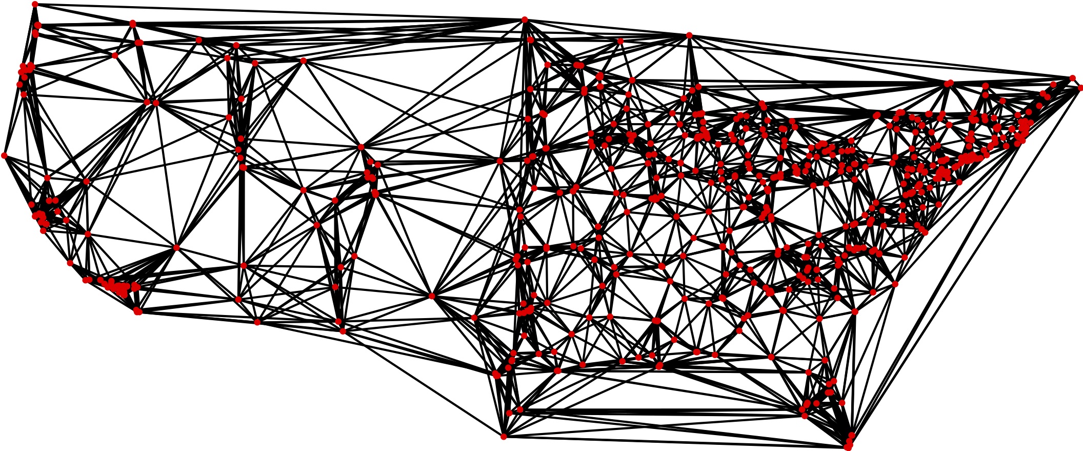
You can find a drawing of the point set without the solution here. But don't spend too much time checking possible routes. The tour we found really is optimal.
![]()
Finding the shortest college tour is an example of the challenge called the traveling salesman problem, or TSP for short. The general problem is a notoriously difficult nut to crack, with a $1,000,000 bounty offered for an efficient solution.
Fortunately, to find the shortest route to visit all of our colleges, we don't need to solve every traveling salesman problem. We only need to solve this particular example.
One 647-city example, versus a whole world of mathematical methods that can be wielded, including 60 years of direct TSP research by a few thousand mathematicians, engineers, and computer scientists. It wouldn't be a good idea to bet on the 647 cities winning the showdown.
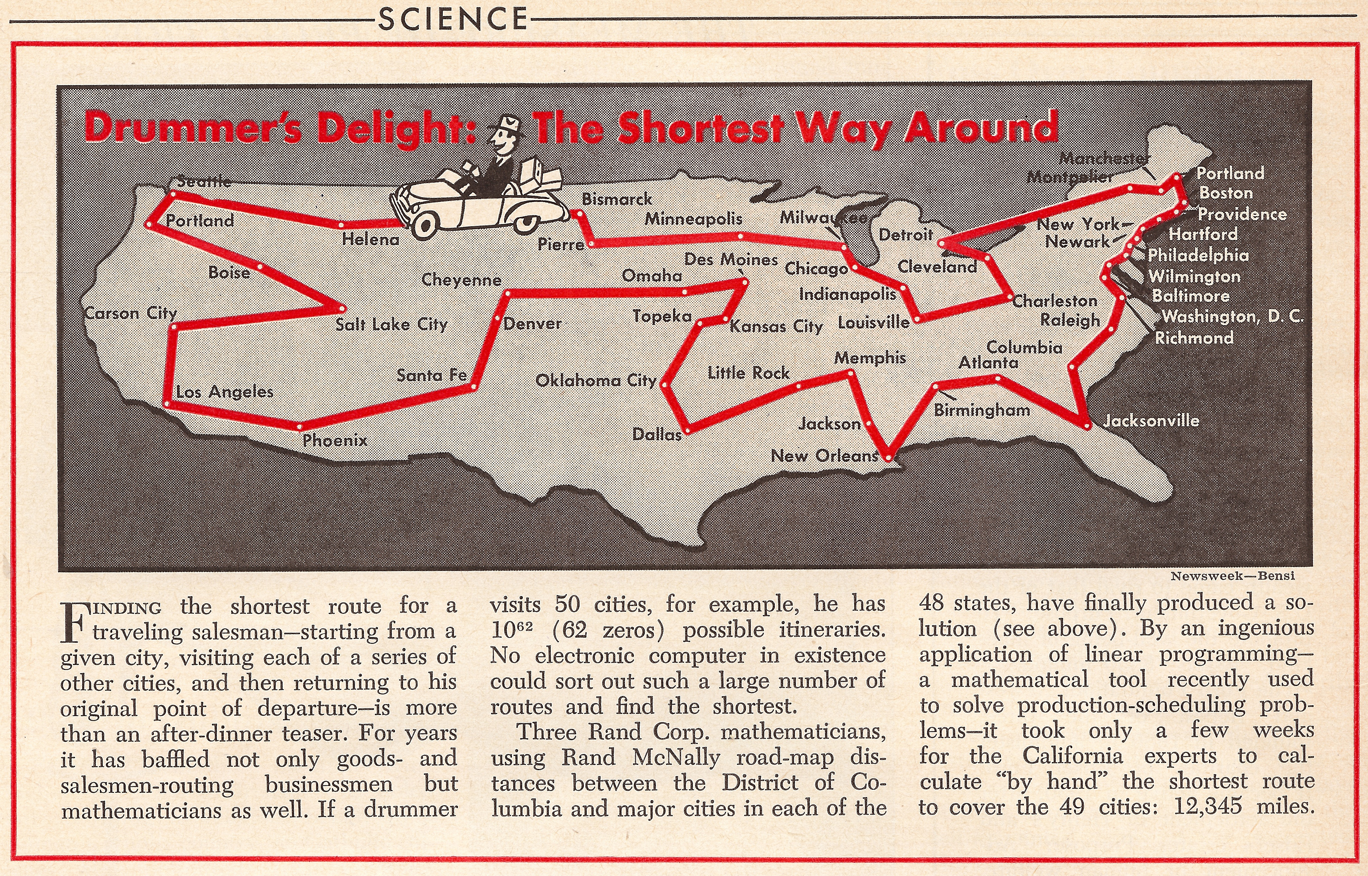
The approach we use for solvling the TSP in our Concorde code goes back to 1954, when it was introduced by George Dantzig, Ray Fulkerson, and Selmer Johnson to tackle a 49-city routing problem.
A high-level description of the Dantzig-Fulkerson-Johnson method is the following: we gather simple rules that all TSP tours must satisfy, find the best result (which might not be a tour) satisfying all of the rules, and repeatedly add more rules until we get a tour. The engine that drives the loop is a device of Dantzig's called linear programming (LP). This engine allows us to use rules such as ``we must choose exactly two roads meeting each college location'' or ``we must choose at least two roads crossing the border into any region of the country that contains at least one of our colleges''. As long as our rules fit into the LP scheme, we can quickly find the best solution satisfying all of them by employing Dantzig's simplex algorithm.
The main word of caution is that an LP model does not allow rules of the form ``either use the route between college A and college B or do not use it.'' In an LP model, we have to permit solutions to potentially use only a fraction of the route between two locations. It is like sending half a salesman in one direction and half in the other direction, a sort of Yoga Bera solution: ``When you come to a fork in the road, take it.'' This, of course, complicates the solution process, but it is the price we pay for having the great speed of the simplex algorithm at our disposal.
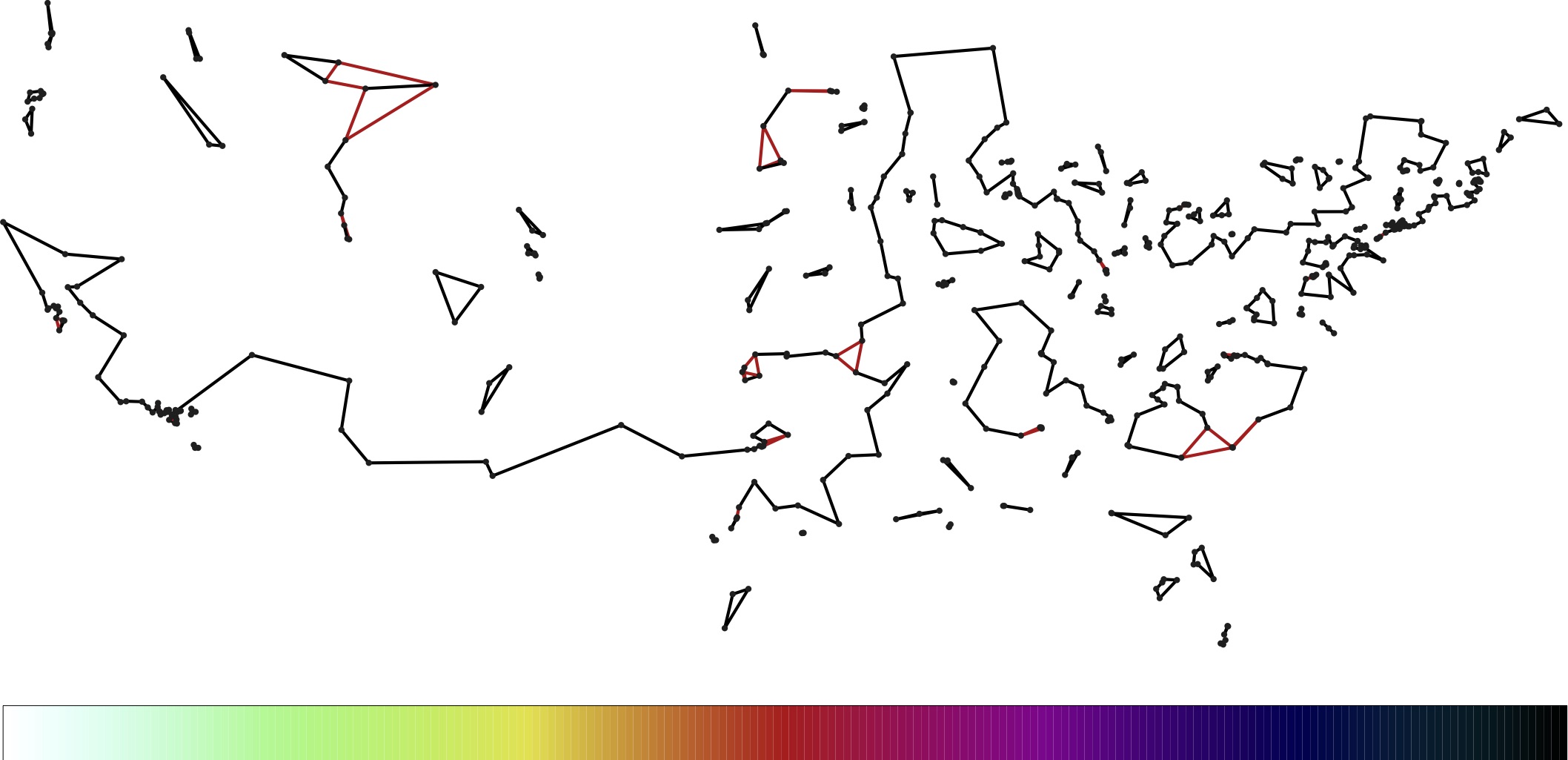
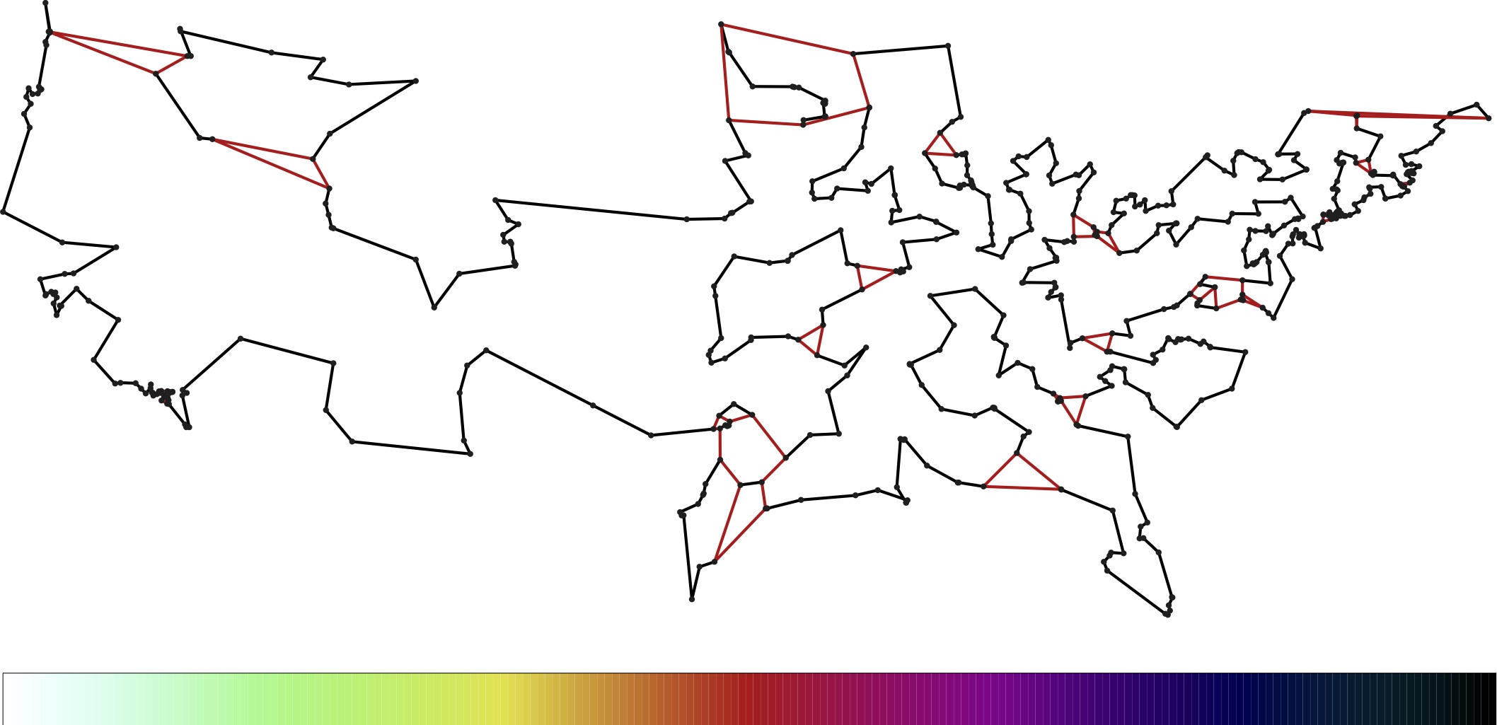
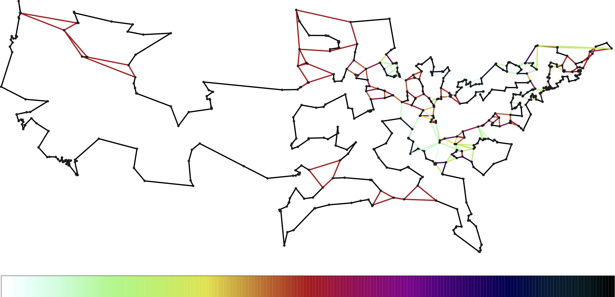
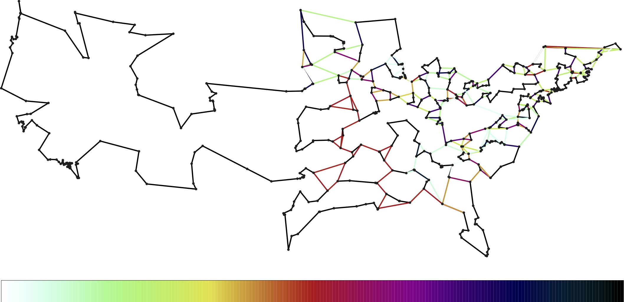
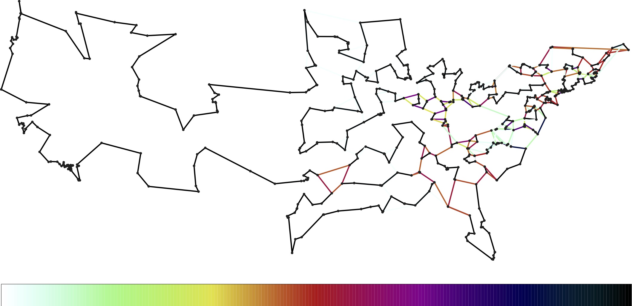
In the set of images below, you can see how the LP solution evolves as we add more and more rules to the model. In the first image, the only rule we used is the one stating that we must choose exactly two roads meeting each location. In LP terms, this means the fractions assigned to the roads meeting the locations must sum to two. To visualize the fractions, we colored roads red if they are set to 1/2, colored them black if they are set to 1, and colored them with values along the indicated scale for any inbetween fractions.
The full process took several hundred steps, but you can get the idea by viewing the five snapshots. Note that the LP solution gets more and more tour-like as we move along.
|
| Initial LP solution. Click for a larger image. |
|
| 2nd LP solution. Click for a larger image. |
|
| 3rd LP solution. Click for a larger image. |
|
| 4th LP solution. Click for a larger image. |
|
| 5th LP solution. Click for a larger image. |
|
|
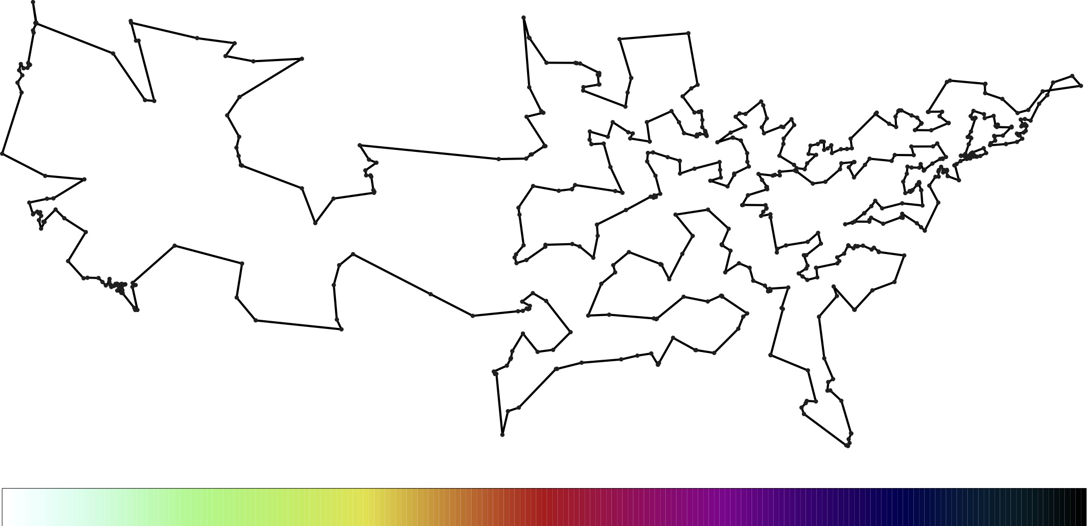
Optimal tour.
Click for a larger image. Note: Tour crossing in Maine is due to travel along roads, rather than by straight lines. |
There are lots of details to get this right, but you can read about all of them in the short book In Pursuit of the Traveling Salesman; the first chapter is available for free. Or, if you would like to see the algorithm running on your own examples, try downloading the free Concorde iPhone/iPad App.
The solution process for the 647-city college tour problem took 290 seconds on my Mac Mini. I can't claim that it can solve every 647-city problem in a reasonable amount of time, but it has handled many, many other examples and research efforts by groups around the world continue to improve the Dantzig-Fulkerson-Johnson technique, year in and year out.
![]()
The traveling salesman problem is a super-clean model. You are handed the distance to travel between each pair of cities and you must find a shortest route to visit them all and return to your starting point. Every example has a correct answer, the challenge is to find it. Preferably before our sun goes supernova.
To bring the TSP to a task like visiting the Forbes' colleges, we need to be able to compute the distance to travel between any pair of them. This point-to-point computation is called the shortest-path problem, one of the easiest models in optimization. Except for one small point. This is where the mathematics of routing comes into contact with the messy world of construction sites, road-surface conditions, traffic jams, and much more.
Dantzig, Fulkerson, and Johnson used a Rand McNally distance table in their classic work. The natural source these days is Google Maps. Google's algorithms weigh a stack of criteria when selecting a point-to-point route. You can sometimes find alternative routes that you might prefer, but, in planning such a long trip, I'm happy to leave the selection in Google's hands.
There is a practical matter, however. To build the full distance table for the 647 colleges, we need to ask for (647 x 646) / 2 = 208981 point-to-point routes. The division by two is because we will just ask for one trip between each pair, rather than asking for directions from both A to B and from B back to A.
The difficulty is that Google allows only 2,500 point-to-point queries per day. Asking for all of the pairs would take over two months, putting our tour planning out of reach for this year's crop of student travelers. So let's see what we can do.
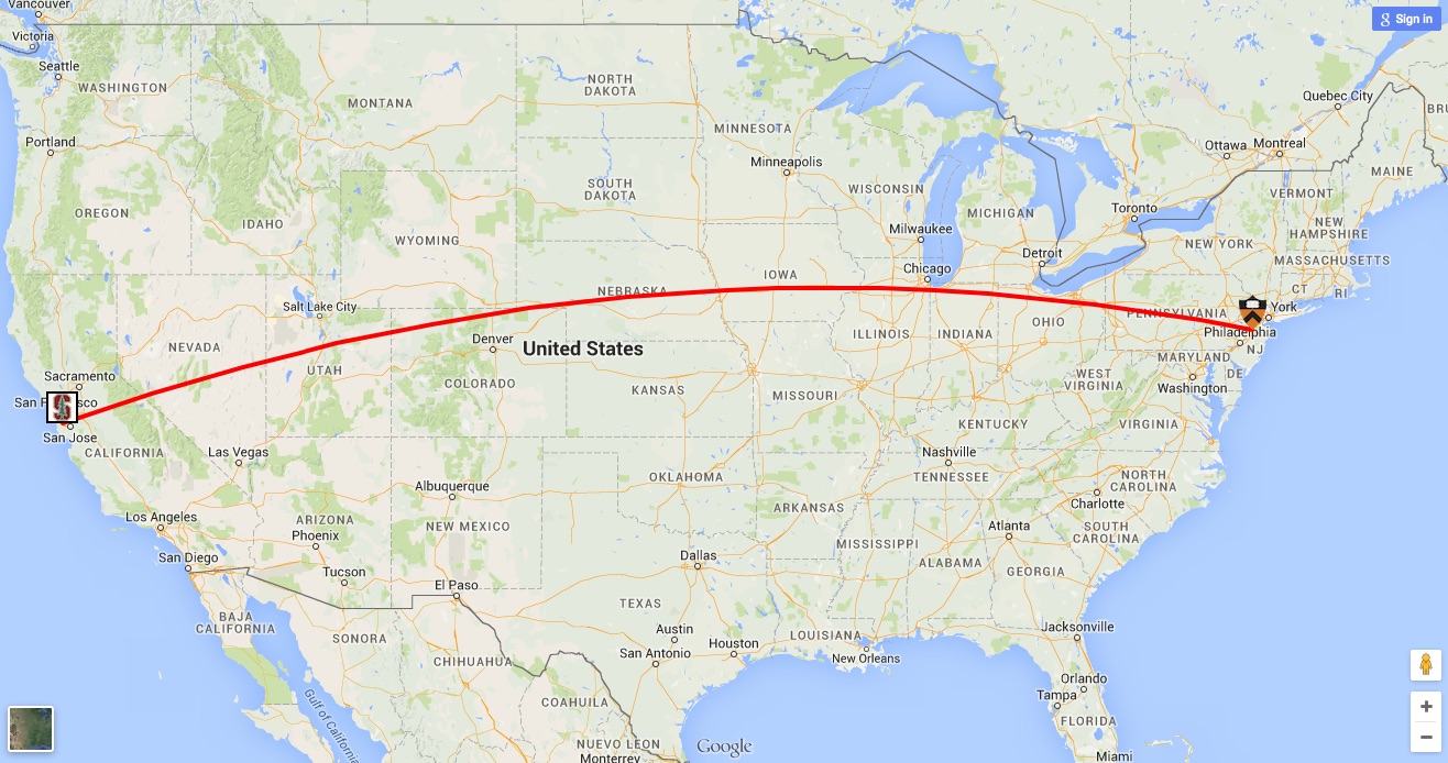
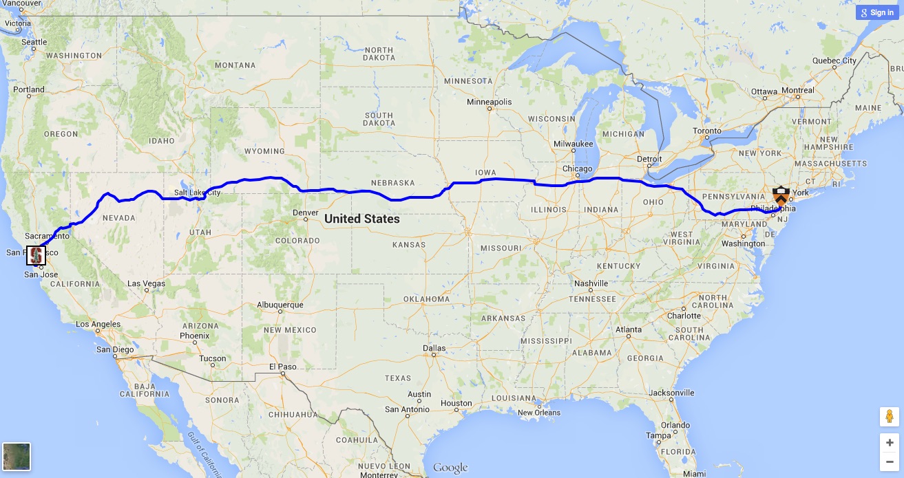
Getting from Princeton to Stanford clocks in at 2,940 miles with Google Maps' road directions. But in a tour through all 647 colleges, we won't likely need to know this route: there are many other campuses between the coasts that we would visit along the way. Indeed, in our computations we can can likely make due with an under-estimate of the Princeton-to-Stanford travel distance, computing the length of a great circle arc on a ball of about the radius of the Earth.
|
|
|
| Great circle estimate: 2536 miles |
|
Using roads: 2940 miles |
Using some geometry, we made an initial guess at what roads might be useful in the college tour, combining a Delaunay triangulation of the point set, the 10 shortest lines from each point, the 2 shortest lines in each of the four quadrants at each point, and the union of 10 near-optimal tours (for the geometric TSP, not the road TSP). Putting these sets together gives the collection of 4,939 campus-to-campus road trips that we display in the graph below.
|
| Initial selection of candidate roads for our tour. Click for a larger image. |
For each of these candidate trips, I asked Google Maps for the recommended route and recorded its length in meters. For all other pairs of colleges, I recorded only the great circle under-estimate of the travel distance to go from one campus to the other.
Concorde quickly solved the resulting TSP, but, sadly, my initial guess at candidate roads was not sufficient. The optimal tour contained 21 of the great-circle trips, and so it was not one we could drive with a non-flying car. But, not to worry, we asked Google for these 21 routes, added them to our candidate list, and solved the problem again.
After 42 rounds of this trial and error, the optimal TSP tour was finally one that used only the Google-supplied road routes. And, with that, the college tour problem was solved. It does not matter that our table of distances contains many great-circle trips, since even with these short cuts we are not using any of the routes in the optimal tour.
The trial-and-error loop added a total of 175 trips to our collection, mostly in the corners of the country.

|
| Additional candidate roads for our tour. Click for a larger image. |
The overall technique can certainly scale up to even larger road trips. Not that anyone really wants to spend a few months out on the road, but what the heck. New challenges can lead to interesting math and engineering. So please drop me a line if you know a couple of thousand nice locations for a TSP tour.
![]()
The general techniques we used to solve the college-tour TSP come from a research area called mathematical optimization. Once every three years, the field's top researchers come together for a week-long conference called the International Symposium on Mathematical Programming, or ISMP for short. The next meeting, ISMP 2015, will be held this July in Pittsburgh.

|
You may have noticed that most articles written about the TSP make a big point to describe how the problem is impossible to solve, usually making a quick calculation about the vast number of possible tours through the point sets. Well, you won't find any of these optimization deniers in Pittsburgh.
When faced with an example of a tough optimization problem, this crowd takes the bull by the horns and finds a way to nonetheless produce a solution. I'm excited to see the progress that has been made since the Berlin ISMP in 2012. If you are interested in optimization, then head to Pittsburgh in July.
![]()
Alternative drawings of the College Tour
![]()
Credits