Appendix

Here we describe the student designed structure implemented for each node shown in Figure . Excluded are those nodes uncompleted and those nodes described in the text above. The structure of each node is separated into three distinct descriptive pieces: initial information displayed, viewed-object, activities available, and signposts.

Summary Stats

Initial display: Scrollable table of summary statistics for each variate in the dataset.
Viewed-object: The dataset.
Activity: None.
Signposts: None. Terminal node.

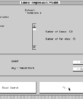
Linear Modelling Hub

Initial display: Dataset summary as in the regression hub and two editable text fields - one for entering the name of the response variate, the other for entering the linear predictor in extended Wilkinson-Rogers notation.
Viewed-object: Linear-modelling-hub
Activity: Editing the model formula to be used by the fit button.
Signposts: 1. ``Model Search'' leading to a corresponding hub (unimplemented) and 2. ``Fit'' which fits the specified model via least-squares and calls display with signposts on the resulting fit-object.

 

Figure 4: Modelling hub

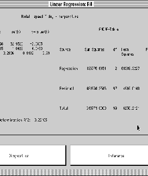
Display of Fit

Initial display: Two tables 1. the estimates, standard deviations, t-statistic for each term in the model and 2. the Anova table including F-statistics and the corrected R² statistic.
Viewed-object: The least-squares fit-object which itself contains pointers to a model-object, the dataset, and calculational details like a QR-decomposition object. The whole hub is simply the result of calling display with signposts on the fit-object which is of interest because fit-objects can appear as viewed-objects of many other views (e.g. the curve displayed in a regression plot).
Activity: None.
Signposts: 1. ``Diagnostics'' and 2. ``Inference''

 

Figure 5: Display of fit

Diagnostic Hub

Initial display: Model formula. Boxplots of each variate in the dataset.
Viewed-object: Linear-regression-assessment object which itself contains pointers to the fit-object.
Activity: None.
Signposts: 1. ``Influential Analysis'', 2. ``Collinearity Analysis'', and 3. ``Residual Analysis''

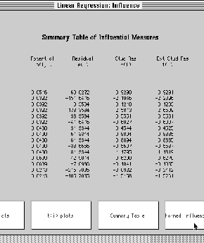
Influential Analysis

Initial display: Table containing case name, h_ii, least-squares residual, studentized residual, and externally studentized residual. The table is scrollable over the cases.
Viewed-object: The fit-object.
Activity: Buttons to replace table display by 1. h_ii vs. i and $\frac{h_{ii}}{1 - h_{ii}}$ vs. t_i (the externally studentized residual), 2. t_i vs. i and $\frac{h_{ii}}{1 - h_{ii}}$ vs. t_i, and 3. Back to the table display.
Signposts: 1. ``Normed Influence Measures''

 

Figure 6: Influence analysis

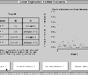
Normed Influence Measures

Initial display: Table showing the mathematical definition of four normed influence measures as described for example in Cook and Weisberg (1983) including ``Cook's distance'' and ``DFFITS'' of Belsley et al (1980).
Viewed-object: The fit-object.
Activity: Four buttons, one for each normed measure in the table. Pressing a button produces an index plot of that measure to the right of the table.
Signposts: None.

 

Figure 7: Normed Influence measures

Collinearity Diagnostics

Initial display: None
Viewed-object: collinearity-hub.
Activity: None.
Signposts: 1. Variance decomposition proportions, 2. Variance inflation factors, and estimators' correlation matrix, 3. Signal to noise testing.

Variance decomposition

Initial display: 1. Table showing, the log₁₀ condition indices and a variance decomposition proportions table (see Belsley et al 1980, Belsley 1991).
2. A scrollable list of the terms in the model.
3. An editable list identifying the terms to be considered as the dependent variate in an examination of auxiliary regressions (see Belsley 1991 for strategy).
4. A list of the auxiliary regression models already determined.
Viewed-object: variance-decomposition object.
Activity: Editing of the terms to be considered dependent in an auxiliary regression analysis.
Signposts: 1. Fit the identified auxiliary regressions.

 

Figure 8: Variance decomposition proportions

Auxiliary regression analysis

Initial display: 1. A list of all fitted auxiliary regression models having the each specified term as the dependent variate.
Viewed-object: auxiliary-regression-analysis.
Activity: Fitted models may be selected.
Signposts: 1. Fit from the currently selected model can be displayed with signposts

V.I.F. and correlation

Initial display: 1. The correlation matrix for the coefficient estimators.
2. The variance inflation factors associated with each coefficient.
Viewed-object: vif-correlation-analysis.
Activity: None.
Signposts: None.

Residual Analysis

Initial display: None.
Viewed-object: The fit-object.
Activity: Offers three different types of residual examination. 1. Gaussian qqplot, 2. Residuals vs. fitted values, and 3.Side by side of (a) residuals versus an explanatory variate in the model and (b) Added variable plot for the effect of the same explanatory variate. Separate buttons produce each of 1,2, or 3 in the display area. A fourth button ``next'' cycles the side-by-side plots of 3 through the explanatory variates in the model one at a time. Plot 3(b) has a ``lowess'' smooth superimposed.
Signposts: None.

 

Figure 9: Residual analysis

Inference Hub

Initial display: None.
Viewed-object: inference-hub.
Activity: None.
Signposts: 1. Hypothesis tests, 2. Confidence Intervals, 3. Prediction Intervals.

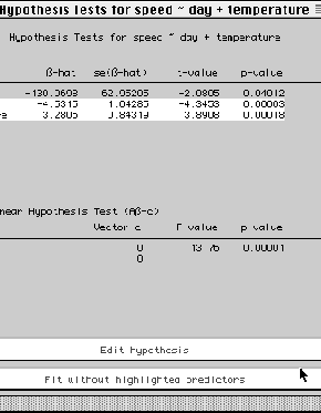
Hypothesis tests

Initial display: 1. Table of estimates, standard errors, t-statistics, and significance levels for each coefficient in the regression.
2. Table of results for testing a general linear hypothesis.
Viewed-object: The fit-object.
Activity: 1. General linear hypothesis of the form ${\boldmath A}~{\boldmath\beta} = {\boldmath c}$ can be tested. User is prompted for the matrix ${\boldmath A}$ and the corresponding vector ${\boldmath c}$. Resulting F-statistic and significance level are then displayed.
2. Selecting terms in the teble of estimates can be tested for simultaneously being zero. Results are displayed in terms of the corresponding general linear hypothesis.
Signposts: None.

 

Figure 10: Hypothesis tests

Confidence Intervals

Initial display: Table of estimates, standard errors, and 95% confidence intervals for each coefficient in the regression.
Viewed-object: The fit-object.
Activity: 1. Change the confidence level.
2. Produce a confidence interval for an arbitrary linear combination of coefficients.
Signposts: None.

Prediction Intervals

Initial display: Table of estimates, standard errors for each coefficient in the regression. A 95% prediction interval and a point prediction for the response at the pre-specified values of the explanatory variate (prompted for at creation).
Viewed-object: The fit-object.
Activity: Change the prediction level.
Signposts: None.