C&O466/666 |
    |
Go to Math Faculty | Go to Combinatorics and Optimization |
Conduct of Course
-
Professor Henry Wolkowicz,
MC 6065, ext. 5589,
-
Numerical Optimization, by
Jorge Nocedal, and
Stephen Wright, 1999,
Springer Verlag.
(
Please look at (and send me any)
typos/comments on the text!
And
more typos at author's website.
)
- Nonlinear Programming, by Dimitri P. Bertsekas, 1999, Athena Scientific.
- Practical Optimization, P.E. Gill, W. Murray, M.H. Wright.
- Numerical Methods for Unconstrained Optimization and Nonlinear Equations, J.E. Dennis and R.B. Schnabel
- Nonlinear Programming: theory and algorithms, M.S. Bazaraa, C.M. Shetty, Sherali
- Linear and Nonlinear Programming, D.G. Luenberger, Second Edition
- Nonlinear Programming, Peressini, Sullivan, Uhl
- Practical Methods of Optimization, R. Fletcher
- Mathematical Programming Methods, G, Zoutendijk
- Nonlinear Programming, G.P. McCormick
- Mathematical programming : theory and algorithms, M. Minoux (QA402.5.M5613)
- Optimization by Vector Space Methods, D.G. Luenberger
- Convex Analysis, R.T. Rockafellar
-
Theory of Extremal Problems, A.D. Ioffe and V.M. Tihomirov
-
will consist of homework problems
.
(See attached schedule of assignments.)
-
A 3-hour exam, date ????.
- Homework............ 50%
- Final Exam.......... 50%
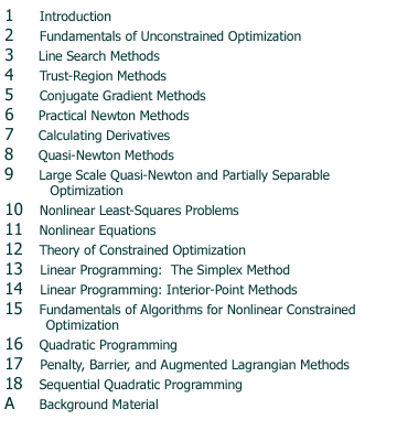
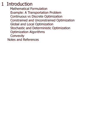
COURSE TOPICS OUTLINE - C &O 466/666

|
 |

|
HOMEWORK LIST- C &O 466/666
-
Homework #1
(Unconstrained Optimization)
Due: Thursday January 13, 2005 (at start of class)
Reading- Chapters 1 and 2 in the text (pages 1-30)
-
For your interest only:
- NEOS Guide Optimization Tree
- You can use MATLAB on many machines on campus. An online course, which works with pretty well any browser that supports the Flash plug-in on Windows, Linux, Solaris, Mac OS is available at: http://saw.uwaterloo.ca/matlab Click: "MATLAB Mastery I" to start.
-
Go to the
NEOS Solvers
web page. Use the unconstrained optimization package CGplus
to solve the extended Rosenbrock function
(see e.g. page 248 in the text or the sample submission
for CGplus) with n=48 variables, parameter values alpha=10 and
alpha=250, and method=2
(Polak-Ribiere).
Then solve the problem using the unconstrained optimization package NMTR.
Hand in (or email in) a copy of the outputs you get by email. In each case, point out the solution and the optimal value. - Pages 30-31, Problems 2.1, 2.3, 2.7, 2.9, 2.15.
-
Homework #2
(Unconstrained Optimization)
Due: Thursday January 27, 2004 (at start of class)
Reading- Chapter 3 in the text (pages 34-61)
- Supplementary Reading (not essential): Sections on Convex Sets and Convex Functions in Introduction to Convex Optimization, course notes by Stephen Boyd, including Lagrangian duality, LP duality, interior-point methods, and semidefinite programming; see also Parts 2,3 in the notes by Lieven Vandenberghe
- For your interest only: Decision Tree for Optimization Software
-
MATLAB
- local MATLAB tutorial (video based)
- Matlab appears to be on all the Solaris systems in the undergrad
environments, e.g. cpu01.student.math and magnus.
You may have to go see Lori Suess in MFCF to set your password properly.
(The path is:
/.software/local/.admin/bins/bin/matlab You should also have an account on (the multiple processor machine) tuxor. The default should now be version matlab-6.5. If not you should try the path software/matlab-6.5/bin/matlab or use "setenv PATH `/bin/showpath matlab-6.5 current`")
Enter the command matlab to start up the matlab session. Then enterhelp optimYou will see a list of the optimization functions that are available with the optimization toolkit. - Now try the command
optdemoThis will bring up a menu. You can try the four choices. The first choice is a tutorial. This demonstrates several of the optimization functions.
- The second choice in the optdemo is the minimization of the banana
function or Rosenbrock's function. This is a classical example of a
function with a narrow valley that exhibits ``very'' slow convergence
for
steepest descent type methods. Try out several methods to minimize this
function.
-
Submit contour and surface plots of the banana function for variable values between
-15,+15 (Use the matlab commands: help plot; or: demo ) - How many function evaluations did the minimization take for: steepest descent; simplex search; Broyden-Fletcher-Golfarb-Shanno; Davidon-Fletcher-Powell; Levenberg-Marquardt? (Please specify the line search you used.)
-
Submit contour and surface plots of the banana function for variable values between
- Pages 62-63, Problems 3.2, 3.3, 3.6, 3.8
- COMMENTS
- Here is a MATLAB code that shows a mesh plot of the extended Rosenbrock function and a plot of the function in the direction of steepest descent at the starting point (-1,-1).
- Here is a MATLAB file with Cauchy's steepest descent for a quadratic function that illustrates both the worst and best case behaviour;
- and here is another simple matlab code for Cauchy's steepest descent with a quadratic function. One can easily change the condition number and see the change in behaviour.
-
Homework #3
(BFGS and Newton; Line Search and Trust Region Techniques)
Due: Tuesday February 15, 2004 (at start of class)
Reading- Chapter 4 in the text (pages 64-97)
- FYI see Lecture 8 on Smooth unconstrained minimization.
-
MATLAB
Solve problem 3.9 on page 63 of the text. But do not program the BFGS algorithm yourself but rather use the matlab function for BFGS, i.e. you can find this by running optdemo and using the information, e.g. lines like
[x,fval,exitflag,output] = fminunc({f,GRAD},x,OPTIONS);
Output the values to verify that they indeed stay positive.
Note: You can modify the matlab programs. You can see what the matlab routines are doing by looking at the matlab m-files. To do this change directory using: cd /software; cd matlab; cd distribution; cd toolbox; cd optim. In particular, there is an m-file called bandemo.m as well as the file fminunc.m - Page 97, Problem 4.1 ( see this MATLAB file for drawing the curve in the problem); Page 99, Problem 4.11.
- Derive the algorithm for the Newton step used in the More-Sorensen
algorithm for the trust region subproblem, as presented in class on Feb.
3, 2005, i.e. in equation (4.27) on page 82.
-
The following MATLAB files might be of interest:
- gentrs.m, generates a random TRS of size n;
- plotrs.m, finds the optimal lambda using a plot of ||p(lambda)||;
- tplottrs.m, finds the optimal lambda using a plot of 1/||p(lambda)||;
- iterN.m finds the optimal lambda using Newton's method (but no safeguarding is included!!!)
- hardcase.m changes g for the hardcase and plots the curves
-
Homework #4
(Constrained Nonlinear Programming and Convex Analysis)
Due: Tuesday March 8, 2004 (at start of class)
Reading- Chapters 12 in the text (pages 314-?)
- For further information on Lagrange Multiplier Theorems and modern proofs see
the paper:
        author    = "B.H. POURCIAU",
         title     = "Modern multiplier methods",
         journal   = "American Mathematical Monthly",
         year      = "1980",
         volume    = "87",
         number    = "6",
         pages     = "433-451"}
This paper is available on campus using JSTOR, e.g. try the link http://www.jstor.org/cgi-bin/jstor/listjournal/00029890/di991653?config=jstor&frame=frame&userID=8161a648@uwaterloo.ca/01cc99331a0050473801&dpi=3
- Constraint Qualifications
- Consider the general NLP with both equality and inequality constraints. Define the tangent cones and the linearizing cones at a feasible point x. Then show that the tangent cone is a subset of the linearizing cone.
-
Consider the NLP:
-
miniminze f(x,y,z)= ex + e-y+z
- Verify that the NLP is a convex program.
- Use the KKT conditions to test for optimality at the origin (0,0,0)T.
- Use the Rockafellar/Pshenichnyi conditions (polar of tangent cone condition) to test for optimality at (0,0,0)T.
- Is there a contradiction between the two tests for optimality? Find the linearizing cone at (0,0,0)T. Then find a direction in the linearizing cone that is not a tangent direction and use this to explain the discrepency.
subject to:-
g1(x,y,z)= ex -1 <= 0
g2(x,y,z)= e-y -1 <= 0
g3(x,y,z)= (x -1)2 + y2 -1 <= 0
g4(x,y,z)= x2+y2+e-z -1 <= 0
-
MATLAB (try to use matlab 7)
- Use the constrained optimization function fmincon in the optimization toolbox to solve the above convex program (problem 1.2 above). Can you get high accuracy in the solution?
- Problems from text:
- Page 359, Problem 12.10
- Page 360, Problem 12.17
-
Homework #5
(Fundamentals of Linear and Nonlinear Programming)
Due: March 17, 2005- Problems from text:
- Chapter 14: Problems 14.1,14.6,14.9,
- Chapter 15: Problems 15.1,15.7
- Chapter 16: Problems 16.1, 16.2
- Chapter 14: Problems 14.1,14.6,14.9,
- Use NEOS to solve the mathematical program in problem 16.9, i.e. use one of the Nonlinearly Constrained Optimization Solvers. (Use each of the three suggested starting points.)
- Problems from text:
-
Homework #6
(Sample Problems for Final Exam)
Due: Do NOT Hand IN.-
Chapter 15: Problems 15.1
Chapter 17: Problems 17.2, 17.3
Chapter 18: Problems 18.1, Describe the Maratos Effect and one possible "fix" for SQP methods.


