Optimization Tips & Tricks
This script contains the examples shown in the webinar titled Optimization Tips and Tricks: Getting Started using Optimization with MATLAB presented live on 21 August 2008. To view the webinar, please go here and click on recorded webinars.
I've tried to make the demos self explanatory in this file. But if something is broken or not clear, please let me know.
To run the demos in this file, you need Optimization Toolbox and Genetic Algorithm and Direct Search Toolbox, which I will refer to as GADS. These files work with Release R2008a. You will also need the Parallel Computing Toolbox to run hte parallel examples. Most demos should work with older releases, but some will require R2008a products. In particular, the parallel optimization examples require it. You can obtain a demo copy from http://www.mathworks.com/products/optimization/tryit.html or http://www.mathworks.com/products/gads/tryit.html
Contents
- Introduction to Optimization - Mt. Washington Demo
- Getting Started - MATLAB Backslash
- Now Solve using lsqnonneg optimization solver
- Constrain the y-intercept
- Working with function handles
- Solve using lsqcurvefit
- Solve using lsqnonlin
- Passing data using function handles with an M-file objective function
- Nested functions
- Nonlinear Optimization and Topology Considerations
- Try a random starting point (uniform distribution grid of 4 points)
- Solve using genetic algorithms
- Solve using simulated annealing
- Solve using pattern search
- Which solver should I choose?
- Using parallel computing with optimization
- Do-it-yourself parallel optimization
- Scaling considerations
- Redefine RPM to have same scale as Pratio
- Tolerances (TolX, TolFun, etc)
- End game
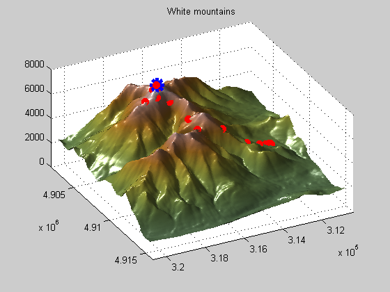
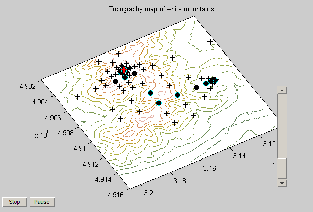
Introduction to Optimization - Mt. Washington Demo
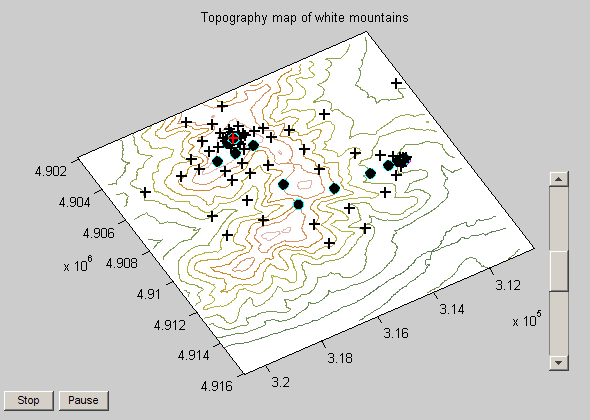
This first example shows you how optimization in general works. Optimization solvers are domain searching algorithms that differ in the types of problems (or domains) they can solve (search). This example shows how the pattern search algorithm can be used to find the peak of the White Mountain Range.
Note: this demo is available in the GADS Toolbox.
% Load data for white mountains
load mtWashington;
% Load psproblem which have all required settings for pattern search
load psproblem;
% Run the solver and show displays
patternsearch(psproblem);

This command will load the example in optimization tool, a graphical user interface for setting up and running optimization problems. You can access optimization tool from the Start Menu --> Toolboxes --> Optimization --> Optimization Tool (optimtool) or by typing optimtool at the command prompt.
% Remove the % symbol if you'd like to run this part of the code.
% mtwashingtondemo
You should see two plots when running the Mt. Washington demo. One is a surface plot, the other is a topology map. On the topology map you can see that starting point and iterations (filled circles) and the tested points that were not selected (+ symbols). There is also a slider bar on the right that you can use to speed up/slow down the process.
Notice how the pattern search solver expands and contracts the search radius as it explores the domain for the maximum value. This is an example of a patterned search, as the name implies, and is only one of many search patterns the pattern search solver supports.
I showed this example to illustrate how effective the pattern search solver can be on a highly rough surface like this one, which gradient based solvers like the ones in Optimization Toolbox couldn't solve.
This leads to the primary difference between the Optimization Toolbox solvers and the GADS solvers. Optimization Toolbox solvers rely on gradients (well, most of them do anyway, fminsearch does not) to determine the search direction. GADS solvers use gradient free methods to find search directions and optimal values. This makes GADS solvers more useful on highly nonlinear, discontinuous, ill-defined, or stochastic problems. They are also better at finding global solutions, although they do not guarantee a global solution will be found.
The price you pay is that the GADS solvers are often slower and are not able to handle as large of problems as the Optimization Toolbox solvers.
Getting Started - MATLAB Backslash
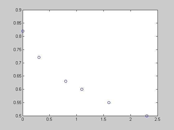
Let's start with a simple curve fitting example. We have time (t) and a response (y). Looking at the plot, you can see that the curve follows an exponential decay.
close all, clear all
t = [0 .3 .8 1.1 1.6 2.3]';
y = [.82 .72 .63 .60 .55 .50]';
plot(t,y,'o')
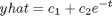
Let's assume that an equation of this from can be used to describe the data
We can linearize this problem and solve it in MATLAB using the backslash operator.
E = [ones(size(t)) exp(-t)]
c = E\y
E =

    1.0000    1.0000
    1.0000    0.7408
    1.0000    0.4493
    1.0000    0.3329
    1.0000    0.2019
    1.0000    0.1003


c =

    0.4760
    0.3413
Notice that we have an over determined system. The neat thing about backslasch (\) is that when you try to solve an over determined system (more equations than unknowns), it tries to minimize the error when estimating the solution. It's an optimization solver (can be used as a least squares minimizer).
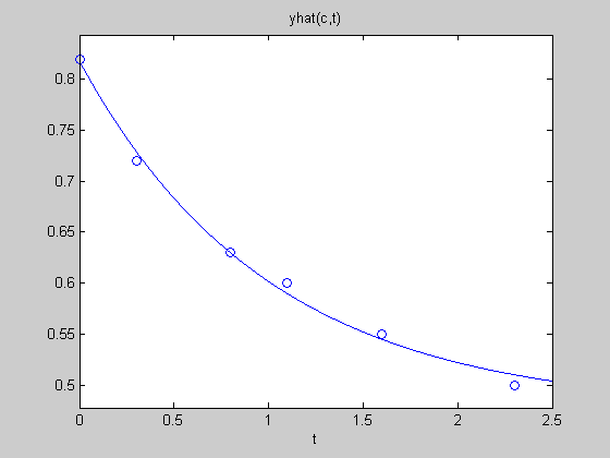
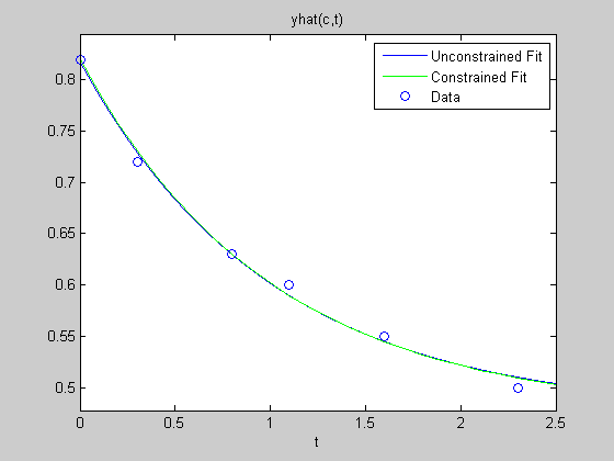
Let's plot the results. Not a bad fit.
yhat = @(c,t) c(1) + c(2)*exp(-t); % I'll describe function handles in a bit
ezplot(@(t)yhat(c,t),[0,2.5])
hold on
plot(t,y,'o')
hold off
Now Solve using lsqnonneg optimization solver
Let's try solving this with an optimization solver. Say lsqnonneg.
c = lsqnonneg(E,y)
c =

    0.4760
    0.3413
We get the same result. Note that lsqnonneg solves a linear system of equations using least squares minimization. If you haven't already, take a look at the optimization documentation for lsqnonneg. And if you have R2008a or later, take a look at the new documentation (Optimization Toolbox --> Optimization Overview --> Choosing a solver). This page gives a nice summary of the optimziation solvers, their problem types, and a decision matrix/table at the bottom of the page. Look at the least-squares solvers and note the different formulations.
That wasn't to hard, but let's now add a constraint to our curve fitting problem and make it a bit more challenging (i.e. something that Curve Fitting Toolbox doesn't currently support.
Constrain the y-intercept
Let's say that we know the data value at time 0 precisely. That is, we can set the starting condition precisely for this exponentially decaying system. This is a constraint, and we can add it to our least squares minimization problem that we've developed so far.
This constraint is a linear constraint on c(1) and c(2). At t = 0, c(1) + c(2)*1 = 0.8 --> Aeq*x = beq --> [1 1][c1 c2]' = 0.8 I've written the constraint in the format accepted by the Optimization Toolbox Solvers. And if we look at the doc for the solver we need, we'd find that the solver that matches our problems is lsqlin.
Aeq = [1 1];
beq = 0.82;
cc = lsqlin(E,y,[],[],Aeq,beq)
Warning: Large-scale method can handle bound constraints only;
    using medium-scale method instead.
Optimization terminated.

cc =

    0.4749
    0.3451
Now let's plot it against our data and the unconstrained fit earlier. We can see that it has a slightly different shape, and if you were to zoom into the y-intercept, you'd see that it passes through our data point where the unconstrained fit did not.
ezplot(@(t)yhat(c,t),[0,2.5])
hold on
tt = 0:0.1:2.5;
plot(tt,yhat(cc,tt),'g')
plot(t,y,'o')
hold off
legend('Unconstrained Fit', 'Constrained Fit', 'Data')
Working with function handles
The solver I showed earlier accepted MATLAB data types, arrays, to define the problem and constraints. However, most of the optimization solvers require that a function be passed in as the objective function(also true for nonlinear constraints). The mechanism that allows you to pass a function into another function is known as a function handle.
A function handle keeps reference to your function and allows you to pass a function into another function.
Let's redefine our equation as an anonymous function (an anonymous function is simply a function that exists only in memory - not in an M-fle).
yhat = @(c,t) c(1) + c(2)*exp(-t)
yhat(cc,t) % pass in the previous solution and the time vector
yhat =

    @(c,t)c(1)+c(2)*exp(-t)


ans =

    0.8200
    0.7305
    0.6299
    0.5897
    0.5445
    0.5095
Note the @ symbol. This declares a function hanlde, and you can see that it behaves like a function call. Note that I can even redefine my function to only take in one input field (this will be important later). Let's redefine yhat to only be a function of c.
yhat2 = @(c) yhat(c,t)
yhat2(cc)
yhat2 =

    @(c)yhat(c,t)


ans =

    0.8200
    0.7305
    0.6299
    0.5897
    0.5445
    0.5095
Notice that when I redefined yhat as yhat2, the time vector t is not passed. How does MATLAB know how to use t in this case? When I redefined the function to accept only c, MATLAB stored the time vector in the function handle object, so it can use it.
To prove this point, notice what happens if I redefine t, yhat2 does not use this new value since it is still referencing the t I had defined at the time I declared yhat2. So t became a constant vector, and was saved with the function handle definition of yhat2.
This is often a point of confusion when first starting to use function handles and it's good to be aware of how parameters get saved when creating a function handle.
t = 0:0.1:2.5; % has more points than before.
y2 = yhat2(cc)
y1 = yhat(cc,t')
y2 =

    0.8200
    0.7305
    0.6299
    0.5897
    0.5445
    0.5095


y1 =

    0.8200
    0.7872
    0.7574
    0.7305
    0.7062
    0.6842
    0.6643
    0.6462
    0.6299
    0.6152
    0.6018
    0.5897
    0.5788
    0.5689
    0.5600
    0.5519
    0.5445
    0.5379
    0.5319
    0.5265
    0.5216
    0.5171
    0.5131
    0.5095
    0.5062
    0.5032
Solve using lsqcurvefit
Ok, so let's get back to the reason I introduced function handles. You need them for most of the nonlinear optimization solvers, as they expect you to pass in a function as the objective or nonlinear constraint.
lsqcurvefit expects a function to be passed in. Here I pass it yhat (note that it is already a function handle in the workspace, if I wanted to pass in an M-file function called yhat, I need to pass it as @yhat). Also take notice that lsqcurvefit allows you to pass in the data to fit to, in this case t and y. You can see we get the same result as in the unconstrained case (this solver does not allow linear constraints, that's why we're using the unconstrained case).
t = [0 .3 .8 1.1 1.6 2.3]';     % define again since we changed it earlier
clear yhat2;                    % no longer needed
c = lsqcurvefit(yhat,[1 1],t,y)
Optimization terminated: first-order optimality less than OPTIONS.TolFun,
 and no negative/zero curvature detected in trust region model.

c =

    0.4760    0.3413
Solve using lsqnonlin
lsqcurvefit is one of the few solvers that let you pass in an objective function with more than one field. But most of our solvers only allow you to pass in one input field - the decision vector. lsqnonlin is an example. Notice in this case that I redefine yhat to be only a function of the decision variables, c. It is also different from yhat2 I defined earlier in that it is subtracting out the y data - i.e. returning only the residuals of the fit. So y and t are passed in as constant parameters to this optimization problem.
This is an example of how you can use function handles to pass in data that your objective function may need to perform a calculation but is considered constant for the optimization problem.
These results agree with prior ones.
c = lsqnonlin(@(c)yhat(c,t)-y,[1 1])
Optimization terminated: first-order optimality less than OPTIONS.TolFun,
 and no negative/zero curvature detected in trust region model.

c =

    0.4760    0.3413
Passing data using function handles with an M-file objective function
This example shows how to pass in the constant data t and y when using a M-file function called myCurveFcn (it's the same as yhat, but in an M-file).
c = lsqnonlin( @(c)myCurveFcn(c,t,y), [1 1])
Optimization terminated: first-order optimality less than OPTIONS.TolFun,
 and no negative/zero curvature detected in trust region model.

c =

    0.4760    0.3413
Nested functions
While function handles are very useful for passing constant parameters, there is another method that works well. This example shows how to use nested function to pass data around in functions. Note that the objective function doesn't get passed t and y into it from the function calling syntax. The nested function has access to it's parent's function workspace, this is where it gets values of t and y that it needs to use in the body of the objective function.
type nestedOptimExample
c = nestedOptimExample()
function c = nestedOptimExample()

% Data
t = [0 .3 .8 1.1 1.6 2.3]';
y = [.82 .72 .63 .60 .55 .50]';

% Curve fitting (Optimization routine)
c = lsqnonlin( @myNestedCurve, [1 1]);

% Objective Function
% Note that t or y are not passed in the function definition
    function resid = myNestedCurve(x)
        yhat = x(1) + x(2)*exp(-t); % where did t come from?
        resid = yhat - y;           % where does y come from?

        % t and y are defined in the parent function but passed to all
        % subfunctions, do not need to pass them explicitly to nested
        % functions.
    end
end

Optimization terminated: first-order optimality less than OPTIONS.TolFun,
 and no negative/zero curvature detected in trust region model.

c =

    0.4760    0.3413
Nonlinear Optimization and Topology Considerations
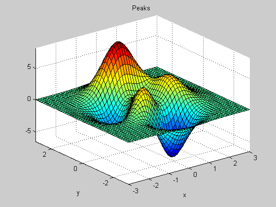
Let's switch gears now, and talk about nonlinear optimization. PEAKS is a function that ships with MATLAB and is shown below. It is a highly nonlinear function and note how close the peaks and valleys are together. This is a very challenging surface to minimize using a gradient based solver, as we'll soon see.
peaks
z =  3*(1-x).^2.*exp(-(x.^2) - (y+1).^2) ...
   - 10*(x/5 - x.^3 - y.^5).*exp(-x.^2-y.^2) ...
   - 1/3*exp(-(x+1).^2 - y.^2)
Let's define our optimization problem. I want to find the minimum value of the PEAKS function. My objective function is the PEAKS function, which I've redefined in a M-file function called peaksObj. It's been redefined here so that it can accept data in the format that the optimization solvers prefer. I'd also like to add a nonlinear constraint to this problem, so you can see how to add them for your problem. I've defined my nonlinear constraint in a function called peaksCon.
clear all, close all
type peaksObj
type peaksCon
function f = peaksObj(x)
%PEAKSOBJ casts PEAKS function to a form accepted by optimization solvers.
%   PEAKSOBJ(X) calls PEAKS for use as an objective function for an
%   optimization solver.  X must conform to a M x 2 or N x 2 array to be
%   valid input.
%
%   Syntax
%      f = peaksObj(x)
%
%   Example
%      x = [ -3:1:3; -3:1:3]
%      f = peaksObj(x)
%
%   See also peaks

% Check x size to pass data correctly to PEAKS
[m,n] = size(x);

if (m*n) < 2
    error('peaksObj:inputMissing','Not enough inputs');
elseif (m*n) > 2 && (min(m,n) == 1) || (min(m,n) > 2)
    error('peaksObj:inputError','Input must have dimension m x 2');
elseif n ~= 2
    x = x';
end

% Objective function
f = peaks(x(:,1),x(:,2));


function [c,ceq] = peaksCon(x)
%PEAKSCON Constraint function for optimization with PEAKSOBJ
%   PEAKSCON(X) is the constraint function for use with PEAKSOBJ.  X is of
%   size M x 2 or 2 x N.
%
%   Sytnax
%      [c,ceq] = peaksCon(x)
%
%   See also peaksobj, peaks

% Check x size to pass data correctly to constraint definition
[m,n] = size(x);
if (m*n) < 2
    error('peaksObj:inputMissing','Not enough inputs');
elseif (m*n) > 2 && (min(m,n) == 1) || (min(m,n) > 2)
    error('peaksObj:inputError','Input must have dimension m x 2');
elseif n ~= 2
    x = x';
end
% Set plot function to plot constraint boundary
try
    mypref = 'peaksNonlinearPlot';
    if ~ispref(mypref)
        addpref(mypref,'doplot',true);
    else
        setpref(mypref,'doplot',true);
    end
catch
end

% Define nonlinear equality constraint
ceq = [];

% Define nonlinear inequality constraint
% x1^2 + x^2 <= 3^2
c = x(:,1).^2 + x(:,2).^2 - 9;
% fmincon accepted input form is ceq <= 0
We'll us the constrained nonlinear minimization solver, fmincon, to solve this problem. Let's define the starting point and solve the problem. (Note that I've created an output plotting function so we can see the solver's iteration history and defined this using solver options).
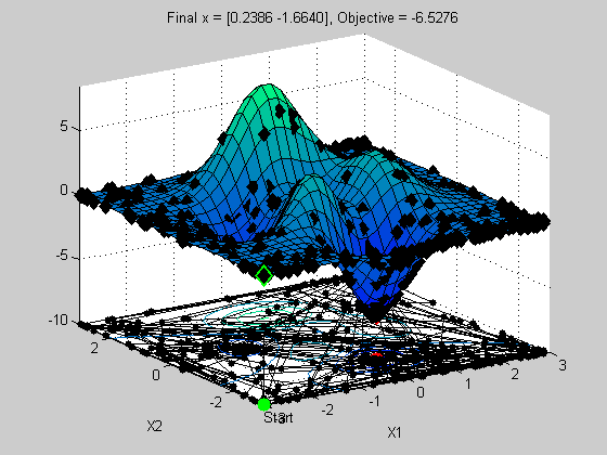
x0 = [0 1.5];
options = optimset('Disp','iter','OutputFcn',@peaksOutputFcn);
x = fmincon(@peaksObj,x0,[],[],[],[],[],[],@peaksCon,options)
Warning: Trust-region-reflective method does not currently solve this type of problem,
 using active-set (line search) instead.

                                Max     Line search  Directional  First-order
 Iter F-count        f(x)   constraint   steplength   derivative   optimality Procedure
    0      3      7.99662        -6.75
    1      6     -3.73667       -7.574            1        -29.3         10.7
    2     11     -4.43864       -4.976         0.25         23.2         22.8  Hessian modified twice
    3     19     -4.44456       -4.667       0.0313           28         19.5
    4     35     -6.14699       -6.299     0.000122     8.4e+003         3.78
    5     38     -6.54458       -6.296            1        0.117          0.5
    6     41     -6.55111       -6.303            1     0.000584       0.0201
    7     44     -6.55113       -6.307            1     1.2e-005       0.0108
    8     47     -6.55113       -6.305            1     4.4e-007      0.00105  Hessian modified
Optimization terminated: magnitude of directional derivative in search
 direction less than 2*options.TolFun and maximum constraint violation
  is less than options.TolCon.
No active inequalities.

x =

    0.2283   -1.6256
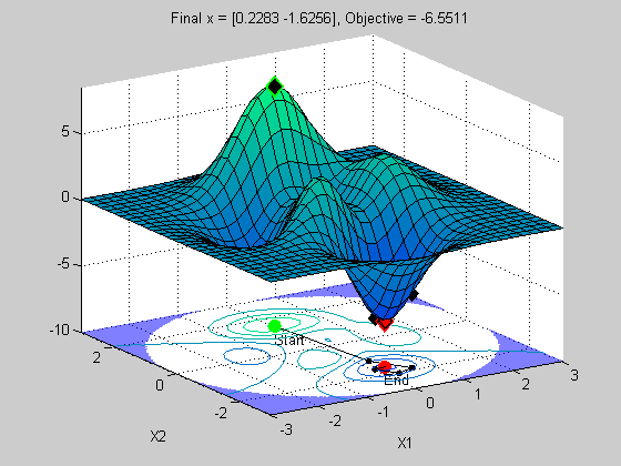
The top plot is a surface plot of the peaks function. The lower plot is a contour plot of the upper plot with the constraint boundary shown in the shaded blue region. This is where we violate the constraint.
Notice how fast it converged to a solution. Looks good right? Let's see what happens when we change the staring point.
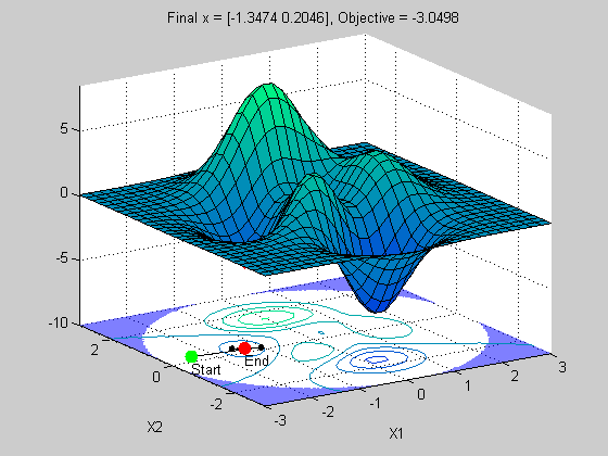
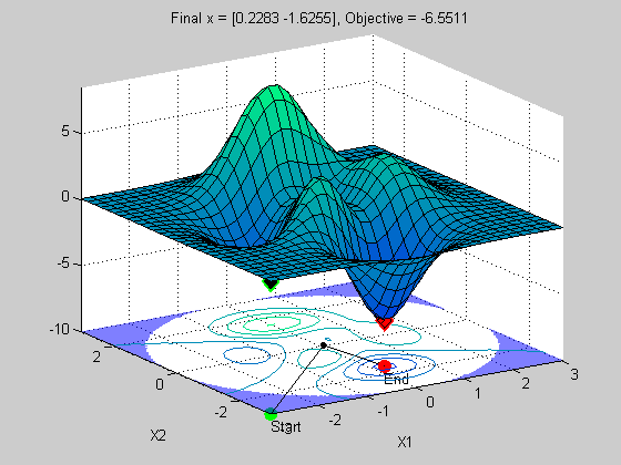
x0 = [-3 -3];
x = fmincon(@peaksObj,x0,[],[],[],[],[],[],@peaksCon,options)
Warning: Trust-region-reflective method does not currently solve this type of problem,
 using active-set (line search) instead.

                                Max     Line search  Directional  First-order
 Iter F-count        f(x)   constraint   steplength   derivative   optimality Procedure
    0      3 6.67128e-005            9                                         Infeasible start point
    1      6    0.0141123        1.125            1       0.0565        0.532
    2      9    0.0263901      0.03138            1       0.0157       0.0175
    3     12    0.0266373    0.0002477            1     0.000238       0.0117
    4     15    0.0144905       0.1616            1      -0.0153       0.0366  Hessian modified twice
    5     18  -0.00406119       0.3202            1      -0.0149         0.31  Hessian modified
    6     24    -0.167801        -1.94        0.125       0.0239        0.673
    7     31    -0.217389       -2.388       0.0625        0.123         0.79
    8     34    -0.862566       -4.674            1       -0.709         1.74
    9     45     -1.19241       -6.091      0.00391         86.2         3.95  Hessian modified
   10     48     -1.85816       -6.444            1       -0.644         3.71
   11     56     -2.90929       -7.486       0.0313         22.8         2.12
   12     59     -3.02511        -7.12            1       0.0704        0.671
   13     62     -3.04903       -7.148            1     -0.00704        0.116
   14     65     -3.04985       -7.144            1   -5.92e-006      0.00879
   15     68     -3.04985       -7.143            1   -4.37e-007     0.000802
Optimization terminated: magnitude of directional derivative in search
 direction less than 2*options.TolFun and maximum constraint violation
  is less than options.TolCon.
No active inequalities.

x =

   -1.3473    0.2045

Bummer! We didn't get the right solution. We did get a local minima, but not the best or global minima. Is this a problem with fmincon? No, this solver was designed to be fast and efficient at finding local minima. It wasn't designed to be a global solver. Most optimization solvers are only local solvers. This is because it is very difficult to guarantee a global solution for nonlinear optimization problems like this one.
This problem also illustrates that the choice of starting point is often critical to finding the right solution.
Try a random starting point (uniform distribution grid of 4 points)
For most practical nonlinear problems, you probably will not run into this issue. But if you suspect that your problem may be this nonlinear, we can get around this starting point issue using multiple staring points (commonly referred to as multistart optimization). Let's do a simple example. I'll run the same optimization problem from four different staring points. How should I choose them? There are a variety of methods you can choose from (such as design of experiments, space filling designs, grid patterns, or any other you can think of). I'm simply going to generate four random starting points ands see how good this works. I'll use a uniform random number generator (all points are equally likely to be selected) and bound the starting points in the range of +/- 3 on each axis.
a = -3;
b = 3;
x1 = a + (b-a) * rand(2);
x2 = a + (b-a) * rand(2);
x0r = [x1; x2];

for i = 1:length(x0r)
    xopt(i,:) = fmincon(@peaksObj,x0r(i,:),[],[],[],[],[],[],@peaksCon,options);
end
xopt
Warning: Trust-region-reflective method does not currently solve this type of problem,
 using active-set (line search) instead.

                                Max     Line search  Directional  First-order
 Iter F-count        f(x)   constraint   steplength   derivative   optimality Procedure
    0      3   -0.0795646      -0.4252
    1      6    -0.413869       -2.275            1       -0.604         1.45
    2     11     -2.56952       -6.502         0.25         72.4          7.4  Hessian modified twice
    3     15     -5.56537       -5.314          0.5         6.81         6.11
    4     22     -5.84013       -5.668       0.0625        0.418         3.92
    5     25     -6.44176       -6.558            1        0.798         2.39
    6     28     -6.54602       -6.248            1       0.0564        0.501
    7     31     -6.55112       -6.303            1    -0.000436       0.0205
    8     34     -6.55113       -6.306            1    5.55e-007     0.000984
Optimization terminated: magnitude of directional derivative in search
 direction less than 2*options.TolFun and maximum constraint violation
  is less than options.TolCon.
No active inequalities.
Warning: Trust-region-reflective method does not currently solve this type of problem,
 using active-set (line search) instead.

                                Max     Line search  Directional  First-order
 Iter F-count        f(x)   constraint   steplength   derivative   optimality Procedure
    0      3   0.00611663         3.08                                         Infeasible start point
    1      6    0.0569658       0.1963            1        0.114        0.161
    2      9    0.0603061     0.006044            1      0.00313        0.053
    3     12    0.0410363      0.08198            1      -0.0174        0.123  Hessian modified
    4     19    0.0198556       0.4217       0.0625       -0.282       0.0935
    5     22    0.0268688      0.09531            1      0.00751       0.0125
    6     25    0.0279356      0.01503            1      0.00104       0.0253
    7     28    0.0279799     0.005353            1    9.12e-006     0.000958  Hessian modified
    8     31    0.0280466     0.001358            1    5.53e-005     0.000208  Hessian modified
    9     34    0.0280769   2.295e-005            1    3.01e-005    2.39e-005  Hessian modified
   10     37    0.0280774   8.225e-008            1    5.24e-007    9.95e-007  Hessian modified
Optimization terminated: first-order optimality measure less
 than options.TolFun and maximum constraint violation is less
 than options.TolCon.
Active inequalities (to within options.TolCon = 1e-006):
  lower      upper     ineqlin   ineqnonlin
                                     1
Warning: Trust-region-reflective method does not currently solve this type of problem,
 using active-set (line search) instead.

                                Max     Line search  Directional  First-order
 Iter F-count        f(x)   constraint   steplength   derivative   optimality Procedure
    0      3      -3.4031       -6.603
    1      9     -5.03052       -5.169        0.125         46.6         6.18
    2     15     -5.22044       -5.843        0.125         3.86         5.42
    3     18     -5.82527       -6.669            1          3.3         3.81
    4     21     -6.53704       -6.221            1        0.221        0.735
    5     24     -6.55099       -6.315            1      0.00183       0.0842
    6     27     -6.55112       -6.304            1    8.92e-005       0.0195
    7     30     -6.55113       -6.305            1    4.86e-007     0.000687  Hessian modified
Optimization terminated: magnitude of directional derivative in search
 direction less than 2*options.TolFun and maximum constraint violation
  is less than options.TolCon.
No active inequalities.
Warning: Trust-region-reflective method does not currently solve this type of problem,
 using active-set (line search) instead.

                                Max     Line search  Directional  First-order
 Iter F-count        f(x)   constraint   steplength   derivative   optimality Procedure
    0      3    -0.390414        -3.09
    1      6     -2.29416       -7.845            1         6.76         4.76
    2     10     -2.71202       -6.502          0.5         2.79         2.44
    3     13     -3.02988       -6.998            1       -0.123        0.745
    4     18     -3.03676       -7.104         0.25       0.0651        0.486
    5     21     -3.04064        -7.21            1       0.0384        0.389
    6     24     -3.04983       -7.138            1     0.000688       0.0242
    7     27     -3.04985       -7.143            1    6.69e-007     0.000986
Optimization terminated: magnitude of directional derivative in search
 direction less than 2*options.TolFun and maximum constraint violation
  is less than options.TolCon.
No active inequalities.

xopt =

    0.2282   -1.6255
    2.7571    1.1824
    0.2282   -1.6256
   -1.3474    0.2046
Now this result will be different each time you run it, but you should see that in this case we found the global minima at least once (possibly more). So multistart can be an effective method for finding the global minima. Also note that I get additional minima when using this method. This may also be useful, depending upon your problem. For example, the global minima may not be a stable condition when you take uncertainty in X1/X2 into consideration and you migh prefer the other minima in this case.
I used only 4 points, but depending upon your problem and the size of your domain you would like to search you may need many more points. So choose your multistart strategy carefully and incorporate any knowledge you may know about your problem to guide you on deciding how many point you need.
Solve using genetic algorithms
One of the benefits of the solvers in the Genetic Algorithm and Direct Search Toolbox is that they are useful for problems that are highly nonlinear, such as this one. They also are useful for problems that are stochastic, contain custom data types such as integer sets, problems that have undefined derivates, holes in the search domain, or are ill-defined. They also are better at finding global solutions than the gradient based solver in Optimization Toolbox.
But they are more expensive and are limited to solving problems of smaller size.
Let's solve this problem using genetic algorithms (GA).
options = gaoptimset('Disp','iter','OutputFcns',@peaksOutputFcn);
x = ga(@peaksObj,2,[],[],[],[],[],[],@peaksCon,options)
                           Best       max        Stall
Generation  f-count        f(x)     constraint  Generations
    1        1060      -6.54929            0      0
    2        2100      -6.55001            0      0
    3        3140      -6.55044            0      0
    4        4180      -6.55087            0      0
    5        5220      -6.55087            0      1
Optimization terminated: average change in the fitness value less than options.TolFun
 and constraint violation is less than options.TolCon.

x =

    0.2279   -1.6213

The plot shows how GA progresses towards a solution. It uses a stochastic search, based upon an initial population of points (green), and the selects a subpopulation (black) for creating a new population to evaluate. GA get's it's name from it's search method, which selectively generate new candidate points to evaluate based upon a method that is similar to breeding among two 'parents' to generate a 'child'. I won't get into the details here, but if you want to know more about GA solvers, I suggest you take a look at our documentation, or watch the Genetic Algorithms for Financial Application Webinar (has a nice description of GA algorithms in it).
You can see that the final population (red) contains the global minima.
Solve using simulated annealing
Another popular solver is Simulated Annealing. This solver is a little more cost effective then GA, but note that it doesn't allow you to solve a problem with nonlinear constraints. But for our problem, we can approximate the nonlinear constraint as a rectangular region, vs. a circular one. So we'll use the lower/upper bounds to add this constraint. Notice how this solver works. It starts out be randomly sampling the domain and gradually reduces the search radius around a mimima that it's found. Periodically, the solver will reset and start searching a wider radius. This is the mechanism that allows this solver to jump out of a local minima and find the global minima.
lb = [-3 -3];
ub = -lb;
options = saoptimset('Display','iter','OutputFcns',@peaksOutputFcn);
x = simulannealbnd(@peaksObj,x0,lb,ub,options)
                           Best        Current           Mean
Iteration   f-count         f(x)         f(x)         temperature
     0          1   6.67128e-005   6.67128e-005            100
    10         11      -0.100733      -0.100733          56.88
    20         21      -0.599882     -0.0186801        34.0562
    30         31       -4.06499     -0.0658076        20.3907
    40         41       -4.06499      0.0220188        12.2087
    50         51       -4.85205   -1.34497e-005        7.30977
    60         61       -4.85205     -0.0297897        4.37663
    70         71       -4.85205    5.7267e-005        2.62045
    80         81       -4.85205     0.00011612        1.56896
    90         91       -4.85205     0.00905351       0.939395
   100        101       -5.96702       -5.96702        0.56245
   110        111       -5.96702       -5.96702        0.33676
   120        121       -5.96702       -5.96702       0.201631
   130        131       -6.54645       -6.54645       0.120724
   140        141       -6.54645       -6.54645      0.0722817
   150        151       -6.54645       -6.52976      0.0432777
   160        161       -6.54645       -6.54053       0.025912
   170        171       -6.55003       -6.55003      0.0155145
   180        181       -6.55045       -6.54975     0.00928908
   190        191       -6.55045       -6.54471     0.00556171
   200        201       -6.55097       -6.54889        0.00333
   210        211       -6.55097       -6.54825      0.0019938
*  219        222       -6.55104       -6.55104        58.0536
   220        223       -6.55104       -3.08855        55.1509
   230        233       -6.55104     -0.0775709        33.0209
   240        243       -6.55104    0.000777385        19.7708
   250        253       -6.55104       -5.45924        11.8375
   260        263       -6.55104    -0.00416131        7.08756
   270        273       -6.55104   -0.000653794        4.24358
   280        283       -6.55104   -0.000455036        2.54079
   290        293       -6.55104       -1.52425        1.52127
   300        303       -6.55104       -1.04489       0.910838

                           Best        Current           Mean
Iteration   f-count         f(x)         f(x)         temperature
   310        313       -6.55104       -5.46296       0.545352
   320        323       -6.55104       -5.66249       0.326522
   330        333       -6.55104       -5.50983       0.195501
   340        343       -6.55104       -6.54819       0.117054
   350        353       -6.55104       -6.45574      0.0700844
   360        363       -6.55104         -6.469      0.0419621
   370        373       -6.55104       -6.49128      0.0251243
   380        383       -6.55104       -6.49261      0.0150428
   390        393       -6.55104       -6.50319      0.0090067
   400        403       -6.55104       -6.54814     0.00539264
   410        413       -6.55104       -6.54864     0.00322877
   420        423       -6.55104       -6.55045     0.00193319
   430        433       -6.55109       -6.55052     0.00115747
   440        443       -6.55109       -6.55088     0.00069302
   450        453        -6.5511        -6.5511    0.000414937
*  455        460       -6.55113       -6.55113        51.9753
   460        465       -6.55113    0.000468286        40.2175
   470        475       -6.55113   -5.52136e-005        24.0797
   480        485       -6.55113     0.00431116        14.4174
   490        495       -6.55113      -0.097089        8.63223
   500        505       -6.55113      -0.120368        5.16843
   510        515       -6.55113       -5.86936        3.09453
   520        525       -6.55113       -2.91456        1.85281
   530        535       -6.55113     0.00881933        1.10935
   540        545       -6.55113       -1.17515       0.664206
   550        555       -6.55113       -1.53236       0.397685
   560        565       -6.55113       -2.13656       0.238109
   570        575       -6.55113       -2.64956       0.142564
   580        585       -6.55113       -2.53638      0.0853586
   590        595       -6.55113       -3.00086      0.0511073
   600        605       -6.55113       -3.02188      0.0305999

                           Best        Current           Mean
Iteration   f-count         f(x)         f(x)         temperature
   610        615       -6.55113       -3.04576      0.0183213
...
Solve using pattern search
Let's now try out pattern search and see how well it does. I explained patternsearch earlier so I won't get into details here. I will however note that this solver's default settings are set to find the local optimum. We'll add a search option that will make it more global.
options = psoptimset('Display','iter','OutputFcns',@peaksOutputFcn,...
                    'CompleteSearch','on','SearchMethod',@searchlhs);
x = patternsearch(@peaksObj,x0,[],[],[],[],[],[],@peaksCon,options)
                                  max
  Iter   f-count      f(x)      constraint   MeshSize      Method
    0     1 6.67128e-005            9       0.9901
    1    70     0.777299            0        0.001   Increase penalty
    2   236     -6.33651            0       1e-005   Increase penalty
    3   438      -6.5511            0       1e-007   Increase penalty
    4   716     -6.55113            0       1e-009   Increase penalty
Optimization terminated: mesh size less than options.TolMesh
 and constraint violation is less than options.TolCon.

x =

    0.2283   -1.6255
Which solver should I choose?
Let's time these approaches and see how they fare.
compareApproaches
Optimization terminated: average change in the fitness value less than options.TolFun
 and constraint violation is less than options.TolCon.


Results from different optimization solvers (default settings):

Solver					Fcn Calls		Time(s)
--------------------------------------------------------------
fmincon (lucky guess)   	47 			0.174108
fmincon (random start)  	189 		0.843512
Genetic Algorithm       	5220 		17.886585
Simulated Annealing     	2406 		1.226381
Pattern Search          	453 		3.991359
From this chart it’s clear that using a gradient based solver, such as fmincon is the best approach. Notice that even if run with a random start, it is still faster than the other methods and often results in fewer function calls. Among the gradient-free methods, we can see that the order of preference in terms of function calls is PS, SA, then GA. And if we considered time to solution, it would be SA, PS, then GA. (Note that I haven't used the vectorize option in these solvers).
Notice that we also can’t necessarily relate function evaluation with time to find the solution when using different solvers. This becomes even more of a consideration when you use parallel computing, which I’ll discuss in a minute. In general, my recommendation is that if you think you have a nonlinear problem like this, or one that you can’t use a gradient based solver on, I’d start with PS as it is typically the most efficient. I’d then use simulated annealing, as it is a compromise between PS and GA and can also handle customized data types, such as integers.
However, GA is likely your best choice if you have custom data types or you have knowledge of the problem that can lend itself to modifying GA’s population selection and modification functions. GA can be efficient if you take the time to set up these functions. I've glossed over the complexity of GA in this demo, and you can tune it to perform better.
Using parallel computing with optimization
Both Optimization Toolbox and Genetic Algorithm and Direct Search Toolbox have built-in support for parallel computing (requires Parallel Computing Toolbox). The built-in support is in selected constrained nonlinear solvers in Optimization Toolbox and Genetic algorithms and Pattern Search solvers in GADS Toolbox.
Let's see how it works. First lets time our objective
tic
peaksObj(x0)
toc
ans =

    7.9966

Elapsed time is 0.004151 seconds.
Let's now run our multistart fmincon example and time it.
clear all, close all, clc
a = -3;
b = 3;
x1 = a + (b-a) * rand(2);
x2 = a + (b-a) * rand(2);
x0r = [x1; x2];

options = optimset('Algorithm','active-set','Display','none');
tic
for i = 1:length(x0r)
    xopt(i,:) = fmincon(@peaksObj,x0r(i,:),[],[],[],[],[],[],@peaksCon,options);
end
toc
Elapsed time is 1.835448 seconds.
And let's rerun it using the build in parallel computing capabilities. Note that to use parallel computing, I need to set an option and open up the matlabpool (start the additional labs). I'm running this on a dual core laptop, so I can use two processing cores (labs) at a time.
options = optimset(options, 'UseParallel','Always');
matlabpool open local 2
tic
for i = 1:length(x0r)
    xopt(i,:) = fmincon(@peaksObj,x0r(i,:),[],[],[],[],[],[],@peaksCon,options);
end
toc
Starting matlabpool using the parallel configuration 'local'.
Waiting for parallel job to start...
Connected to a matlabpool session with 2 labs.
Elapsed time is 2.548319 seconds.
Hey, what gives? This doesn't provide me any benefit!
True, the built-in support is only useful for objective function and/or nonlinear constraint functions that are computationally intensive. What constitutes an expensive function relies a lot on your local network and hardware, but a general rule of thumb is that if your objective function executes on the order of a few hundred milliseconds, you'll probably benefit from using parallel computing.
Let's tweak my problem so it is expensive. I've added a line of code to peaksOjb that simply takes time to compute (if you're interested, it's in the file peaksObjExp).
Time it again.
tic
peaksObjExp(x0r(1,:));
toc
Elapsed time is 0.799754 seconds.
We need to rerun the base case since we are using a different objective function.
options = optimset(options, 'UseParallel','Never');
tic
for i = 1:length(x0r)
    x = fmincon(@peaksObjExp,x0r(i,:),[],[],[],[],[],[],@peaksCon,options);
end
toc
Elapsed time is 41.643885 seconds.
And let's see if we get an improvement using my two cores.
options = optimset(options, 'UseParallel','Always');
tic
for i = 1:length(x0r)
    x = fmincon(@peaksObjExp,x0r(i,:),[],[],[],[],[],[],@peaksCon,options);
end
toc
Elapsed time is 35.457548 seconds.
You can see that I was able to get roughly a 15% improvement. This improvement wasn't bad considering I have one machine with two cores that share the same memory. You'd probably be able to get a better result using more cores or more computers in a cluster.
Let's now take a look at how you could do even better by exploiting the nature of this problem using parallel computing on the for loop.
Do-it-yourself parallel optimization
The built-in parallel computing support in fmincon accelerates the estimation of gradients. While this helped to speed up the solution time, keep in mind that each iteration is dependent upon the previous iteration's results. In other words, there are limits to how much parallel computing can speed up a gradient based solver since it contains serial operations that can't be parallelized.
This problem can benefit form using parallel computing in a different way. Notice that the optimization is being performed four times (the for loop). Each loop is independent of the others, so we can make use of parallel computing in this case, and the Parallel Computing Toolbox makes this easy with the parfor language construct.
options = optimset(options, 'UseParallel','Never');
tic
parfor i = 1:length(x0r)% Notice the for loop is changed to parfor
    x = fmincon(@peaksObjExp,x0r(i,:),[],[],[],[],[],[],@peaksCon,options);
end
toc
Elapsed time is 32.111325 seconds.
You can see that the solution time was reduced by more than 30%. I've showed this method to illustrate that you may benefit from using parallel computing directly in your problems, rather than relying on our built-in solution in some cases. If you do have an expensive objective function, you might be able to use parallel computing in the definition of your objective function to get better performance than using the built-in support. Often the expense arises in the objective function evaluation, and if you can speed that up you'll see the benefit in the optimization solver performance.
clear all, close all, clc
matlabpool close
Sending a stop signal to all the labs...
Waiting for parallel job to finish...
Performing parallel job cleanup...
Done.
Scaling considerations
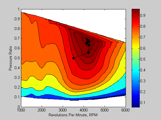
I'd like to show you some additional considerations when working with optimzation. When solving problems, you should pay attention to the magnitude of the decision variables and the objective functions. If there is a wide range, this can impact how the solver proceeds to a solution (numerical issues). Let's look at the case where I have two decision variables of different magnitudes. The plot below shows an engine performance map. The axes show engine speed in RPM and the intake pressure ratio. The color contours are a measure of engine efficiency. Note how the magnitude of the engine speed is nearly 10,000 times that of the pressure ratio. This can present a problem for an optimization solver.
load VEdata
VEPlot([3500 0.5]);

If you think about this magnitude difference in terms of how a gradient based solver searches using derivatives of the objective function with respect to the decision variables, we get a large difference in the change seen due to the magnitude of decision variables (i.e. df/dx1 ~1/1000, df/dx2 ~1/0.1). This large difference leads to numerical problems, and as we see in this example, the optimization solver doesn't progress towards the solution.
options = optimset('Disp','Iter','Algorithm','interior-point',...
                   'OutputFcn',@VEPlot);
objFun = @(x)-VEMap(x,RPM,Pratio,VE);
x0 = [3500 0.5];
lb = [1000 0 ];
ub = [6000 1.0];
tic
z = fmincon(objFun,x0,[],[],[],[],lb,ub,[],options)
toc
                                         First-order     Norm of
 Iter F-count         f(x)  Feasibility   optimality        step
    0     5  -8.963084e-001   0.000e+000   1.071e-001
    1     8  -9.156335e-001   0.000e+000   4.956e-002  1.071e-001
    2    12  -9.324939e-001   0.000e+000   6.138e-002  1.128e-001
    3    18  -9.380426e-001   0.000e+000   2.470e-002  3.484e-002
    4    24  -9.382448e-001   0.000e+000   1.548e-001  1.067e-002
    5    27  -9.384511e-001   0.000e+000   6.813e-003  4.124e-003
    6    30  -9.384536e-001   0.000e+000   5.860e-003  2.930e-004
    7    34  -9.384598e-001   0.000e+000   5.846e-003  7.286e-004
    8    44  -9.384614e-001   0.000e+000   1.800e-003  1.821e-004
    9    55  -9.384620e-001   0.000e+000   1.799e-003  7.960e-005
   10    69  -9.384621e-001   0.000e+000   1.799e-003  4.352e-006
   11    80  -9.384621e-001   0.000e+000   1.799e-003  1.904e-006
   12    92  -9.384621e-001   0.000e+000   1.799e-003  4.164e-007
   13   106  -9.384621e-001   0.000e+000   6.895e-002  2.277e-008
Optimization terminated: current point satisfies constraints and relative
change in x is less than options.TolX.

z =

  1.0e+003 *

    3.5000    0.0008

Elapsed time is 17.487496 seconds.

Redefine RPM to have same scale as Pratio
It is good practice to define your optimization problems such that the magnitudes of the objective/constraint functions and decision variables are of similar magnitude. In this example, I rescaled the decision variables to be of a similar magnitude. I've also changed the objective function definition to accept the scaled decision variables.
Notice that when the problem is scaled correctly, we get the right solution.
close(gcf)
options = optimset('Disp','Iter','Algorithm','interior-point',...
                   'OutputFcn',@(x,o,s)VEPlot([x(1)*10000 x(2)],o,s));
objFun = @(x)-VEMap([x(1)*10000 x(2)],RPM,Pratio,VE);
x0 = [3500/10000 0.5];
lb = [1000/10000 0 ];
ub = [6000/10000 1.0];
tic
z = fmincon(objFun,x0,[],[],[],[],lb,ub,[],options)
toc
                                         First-order     Norm of
 Iter F-count         f(x)  Feasibility   optimality        step
    0     5  -8.963084e-001   0.000e+000   4.366e-001
    1     9  -9.553156e-001   0.000e+000   4.404e-001  9.015e-002
    2    13  -9.631107e-001   0.000e+000   3.441e-001  7.976e-002
    3    16  -9.639381e-001   0.000e+000   1.002e-001  2.053e-002
    4    20  -9.661179e-001   0.000e+000   2.729e-001  3.795e-002
    5    23  -9.702423e-001   0.000e+000   4.237e-001  2.313e-002
    6    27  -9.723160e-001   0.000e+000   6.661e-001  8.627e-003
    7    31  -9.731487e-001   0.000e+000   7.639e-002  5.586e-003
    8    35  -9.732677e-001   0.000e+000   3.384e-001  2.739e-003
    9    38  -9.732614e-001   0.000e+000   1.608e-001  1.757e-003
   10    41  -9.732861e-001   0.000e+000   1.515e-001  2.618e-004
   11    47  -9.733193e-001   0.000e+000   1.572e-001  2.427e-004
   12    61  -9.733199e-001   0.000e+000   1.051e-001  4.199e-006
   13    72  -9.733201e-001   0.000e+000   1.145e-001  1.837e-006
   14    75  -9.733570e-001   0.000e+000   2.016e-001  5.554e-004
   15    80  -9.734154e-001   0.000e+000   2.691e-001  8.766e-004
   16    92  -9.734183e-001   0.000e+000   1.988e-001  5.462e-005
   17   107  -9.734184e-001   0.000e+000   5.276e-002  3.508e-007
   18   110  -9.734161e-001   0.000e+000   2.696e-001  4.706e-005
   19   113  -9.734165e-001   0.000e+000   3.431e-001  6.377e-006
   20   116  -9.734182e-001   0.000e+000   3.420e-001  2.521e-005
   21   126  -9.734186e-001   0.000e+000   9.745e-002  6.302e-006
   22   143  -9.734186e-001   0.000e+000   1.983e-001  8.029e-008
   23   147  -9.734186e-001   0.000e+000   1.983e-001  4.308e-008
   24   154  -9.734187e-001   0.000e+000   1.983e-001  9.129e-008
   25   158  -9.734187e-001   0.000e+000   1.983e-001  6.031e-007
   26   172  -9.734187e-001   0.000e+000   9.729e-002  7.010e-009
Optimization terminated: current point satisfies constraints and relative
change in x is less than options.TolX.

z =

    0.4244    0.6689

Elapsed time is 25.217529 seconds.
Tolerances (TolX, TolFun, etc)
Since we're on the topic of magnitudes, let's return to the Mt. Washington example. Notice the scale of the axes, 1,000s of feet. Also note that we are seeking the peak, which is also in 1,000s of feet. If we run this problem with default settings, we'll get the right solution but it will take 68 iterations to do so.
clear all, close all
% Load data for white mountains
load mtWashington;
% Load psproblem which have all required settings for pattern search
load psproblem;
% show iteration history
psproblem.options.Display = 'iter';
% Run the solver and show displays
patternsearch(psproblem);
Iter     f-count          f(x)      MeshSize     Method
    0        1        -2392.5            10
    1        5       -2396.17            20     Successful Poll
    2        9        -2401.5            40     Successful Poll
    3       13       -2409.58            80     Successful Poll
    4       17          -2428           160     Successful Poll
    5       21       -2462.75           320     Successful Poll
    6       25       -2593.67           640     Successful Poll
    7       29       -2958.83          1280     Successful Poll
    8       33       -4574.17          2560     Successful Poll
    9       37       -4574.17          1280     Refine Mesh
   10       41       -4956.11          2560     Successful Poll
   11       45       -4956.11          1280     Refine Mesh
   12       49       -5138.08          2560     Successful Poll
   13       53       -5194.89          5120     Successful Poll
   14       57       -5194.89          2560     Refine Mesh
   15       61       -5194.89          1280     Refine Mesh
   16       65          -5687          2560     Successful Poll
   17       69          -5687          1280     Refine Mesh
   18       73          -5687           640     Refine Mesh
   19       77       -5767.33          1280     Successful Poll
   20       81       -5767.33           640     Refine Mesh
   21       85       -6052.19          1280     Successful Poll
   22       89       -6052.19           640     Refine Mesh
   23       93       -6052.19           320     Refine Mesh
   24       97       -6172.67           640     Successful Poll
   25      101       -6172.67           320     Refine Mesh
   26      105       -6172.67           160     Refine Mesh
   27      109       -6261.25           320     Successful Poll
   28      113       -6261.25           160     Refine Mesh
   29      117       -6261.25            80     Refine Mesh
   30      121        -6271.5           160     Successful Poll

Iter     f-count        f(x)       MeshSize      Method
   31      125        -6271.5            80     Refine Mesh
   32      129        -6271.5            40     Refine Mesh
   33      133       -6275.53            80     Successful Poll
   34      137       -6275.53            40     Refine Mesh
   35      141       -6276.06            80     Successful Poll
   36      145       -6276.06            40     Refine Mesh
   37      149       -6276.06            20     Refine Mesh
   38      153       -6278.75            40     Successful Poll
   39      157       -6278.75            20     Refine Mesh
   40      161       -6278.75            10     Refine Mesh
   41      165       -6278.81            20     Successful Poll
   42      169       -6278.81            10     Refine Mesh
   43      173       -6278.81             5     Refine Mesh
   44      177          -6280            10     Successful Poll
   45      181          -6280             5     Refine Mesh
   46      185          -6280           2.5     Refine Mesh
   47      189          -6280          1.25     Refine Mesh
   48      193          -6280         0.625     Refine Mesh
   49      197          -6280        0.3125     Refine Mesh
   50      201          -6280        0.1563     Refine Mesh
   51      205          -6280       0.07813     Refine Mesh
   52      209          -6280       0.03906     Refine Mesh
   53      213          -6280       0.01953     Refine Mesh
   54      217          -6280      0.009766     Refine Mesh
   55      221          -6280      0.004883     Refine Mesh
   56      225          -6280      0.002441     Refine Mesh
   57      229          -6280      0.001221     Refine Mesh
   58      233          -6280     0.0006104     Refine Mesh
   59      237          -6280     0.0003052     Refine Mesh
   60      241          -6280     0.0001526     Refine Mesh

Iter     f-count        f(x)       MeshSize      Method
   61      245          -6280    7.629e-005     Refine Mesh
   62      249          -6280    3.815e-005     Refine Mesh
   63      253          -6280    1.907e-005     Refine Mesh
   64      257          -6280    9.537e-006     Refine Mesh
   65      261          -6280    4.768e-006     Refine Mesh
   66      265          -6280    2.384e-006     Refine Mesh
   67      269          -6280    1.192e-006     Refine Mesh
   68      273          -6280     5.96e-007     Refine Mesh
Optimization terminated: mesh size less than options.TolMesh.

If you take a look at the default settings for the tolerances on the objective function (TolFun) and on the decision variables (TolX) you'll note that it is 1e-6. I don't need tolerances anywhere near this tight since my problem is in 1,000s of feet. I doubt my elevation data is even this accurate. This is unnecessary and you can significantly speed up the optimization solver performance by adjusting these parameters to be closer to the accuracy required for the problem. In this case, I'll set the TolFun to 10 (feet), and rerun the solver. We can see that the iterations have been reduced to 43, nearly a 40% reduction.
psproblem.options.TolFun
psproblem.options.TolX

% Adjust the tolerance
psproblem.options.TolFun = 10;

% Run the solver and show displays
patternsearch(psproblem);
ans =

  1.0000e-006


ans =

  1.0000e-006


Iter     f-count          f(x)      MeshSize     Method
    0        1        -2392.5            10
    1        5       -2396.17            20     Successful Poll
    2        9        -2401.5            40     Successful Poll
    3       13       -2409.58            80     Successful Poll
    4       17          -2428           160     Successful Poll
    5       21       -2462.75           320     Successful Poll
    6       25       -2593.67           640     Successful Poll
    7       29       -2958.83          1280     Successful Poll
    8       33       -4574.17          2560     Successful Poll
    9       37       -4574.17          1280     Refine Mesh
   10       41       -4956.11          2560     Successful Poll
   11       45       -4956.11          1280     Refine Mesh
   12       49       -5138.08          2560     Successful Poll
   13       53       -5194.89          5120     Successful Poll
   14       57       -5194.89          2560     Refine Mesh
   15       61       -5194.89          1280     Refine Mesh
   16       65          -5687          2560     Successful Poll
   17       69          -5687          1280     Refine Mesh
   18       73          -5687           640     Refine Mesh
   19       77       -5767.33          1280     Successful Poll
   20       81       -5767.33           640     Refine Mesh
   21       85       -6052.19          1280     Successful Poll
   22       89       -6052.19           640     Refine Mesh
   23       93       -6052.19           320     Refine Mesh
   24       97       -6172.67           640     Successful Poll
   25      101       -6172.67           320     Refine Mesh
   26      105       -6172.67           160     Refine Mesh
   27      109       -6261.25           320     Successful Poll
   28      113       -6261.25           160     Refine Mesh
   29      117       -6261.25            80     Refine Mesh
   30      121        -6271.5           160     Successful Poll

Iter     f-count        f(x)       MeshSize      Method
   31      125        -6271.5            80     Refine Mesh
   32      129        -6271.5            40     Refine Mesh
   33      133       -6275.53            80     Successful Poll
   34      137       -6275.53            40     Refine Mesh
   35      141       -6276.06            80     Successful Poll
   36      145       -6276.06            40     Refine Mesh
   37      149       -6276.06            20     Refine Mesh
   38      153       -6278.75            40     Successful Poll
   39      157       -6278.75            20     Refine Mesh
   40      161       -6278.75            10     Refine Mesh
   41      165       -6278.81            20     Successful Poll
   42      169       -6278.81            10     Refine Mesh
   43      173       -6278.81             5     Refine Mesh
Optimization terminated: change in the function value less than options.TolFun.

End game
This concludes the examples shown in the webinar (plus some additional ones). I hope you enjoyed them and learned something new along the way.