UW Home
  Archimedes’ Sandbox   News and Events   Careers   About Us
math home
contact us
search
directories
depts/schools
popular pages
  Faculty
  Staff
  Graduate Students
  Administration
  Departments
  Research Institutes
  Research Groups
  Computing Services
  Professional Societies
  UW Dir Service
  Women in Math
  Applied Mathematics
  Combinatorics and Optimization
  School of Computer Science
  Pure Mathematics
  Statistics and Actuarial Science
  Canadian Math Competition
  Course Home Pages
  Math Tutorial Centre
  Undergraduate Programs of Study
  Users on www.math.uwaterloo.ca
  Users on www.student.math.uwaterloo.ca

CO466/666
Winter 2004

Continuous Optimization
Course Information


Go to Math Faculty   |  Go to Combinatorics and Optimization

Conduct of Course

  • Instructor:
  • Office Hours:
  • Lectures:
  • Text:
  • Additional References:
    1. Nonlinear Programming, by Dimitri P. Bertsekas, 1999, Athena Scientific.
    2. Practical Optimization, P.E. Gill, W. Murray, M.H. Wright.
    3. Numerical Methods for Unconstrained Optimization and Nonlinear Equations, J.E. Dennis and R.B. Schnabel
    4. Nonlinear Programming: theory and algorithms, M.S. Bazaraa, C.M. Shetty, Sherali
    5. Linear and Nonlinear Programming, D.G. Luenberger, Second Edition
    6. Nonlinear Programming, Peressini, Sullivan, Uhl
    7. Practical Methods of Optimization, R. Fletcher
    8. Mathematical Programming Methods, G, Zoutendijk
    9. Nonlinear Programming, G.P. McCormick
    10. Mathematical programming : theory and algorithms, M. Minoux (QA402.5.M5613)
    11. Optimization by Vector Space Methods, D.G. Luenberger
    12. Convex Analysis, R.T. Rockafellar
    13. Theory of Extremal Problems, A.D. Ioffe and V.M. Tihomirov

  • Course Home Page, C&O 466/666, http://orion.uwaterloo.ca/~hwolkowi/henry/teaching/w04/666.w04/readme.html
  • Term Work:
  • Final Exam:
      A 3-hour exam, ????.
      (Please see the detailed course outline for topics covered during the semester.)
  • Marking Scheme:
    • Homework............ 50%
    • Final Exam.......... 50%

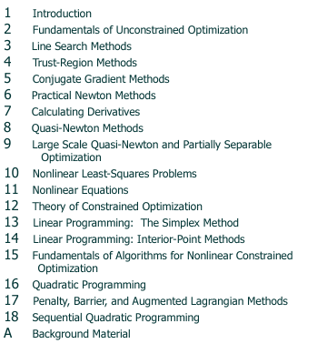
    COURSE TOPICS OUTLINE - C &O 466/666

    We will choose topics from the text. The complete list is included for now.


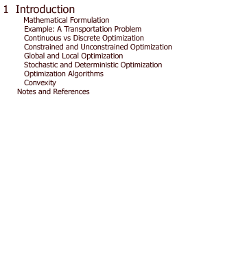
    Background Material Chapter Fifteen Chapter Fourteen Chapter Thirteen Chapter Twelve Chapter Eleven Chapter Ten Chapter Nine Chapter Eight Chapter Seven Chapter Six Chapter Five Chapter Four Chapter Three Chapter Two Chapter Eighteen Chapter Seventeen Chapter Sixteen Chapter One


    HOMEWORK LIST- C &O 466/666

    1. Homework #1 (Unconstrained Optimization)
      Due: Thursday January 15, 2004 (at start of class)
      Reading
      Problems
      • Go to the NEOS Solvers web page. Use the unconstrained optimization package CGplus to solve the extended Rosenbrock function (see e.g. page 248 in the text or the sample submission for CGplus) with n=38 variables, parameter values alpha=12 and alpha=200, and method=2 (Polak-Ribiere).
        Then solve the problem using the unconstrained optimization package NMTR.
        Hand in (or email in) a copy of the outputs you get by email. In each case, point out the solution and the optimal value.
      • Pages 30-31, Problems 2.1, 2.3, 2.7, 2.9.

    2. Homework #2 (Unconstrained Optimization)
      Due: Thursday January 29, 2004 (at start of class)
      Reading Problems
      1. MATLAB
        1. Matlab appears to be on all the Solaris systems in the undergrad and grad environments, e.g. pythagoras, hopper, hermite and magnus. (The path is:
          /.software/local/.admin/bins/bin/matlab
          You should also have an account on (the multiple processor machine) tuxor. The default should now be version matlab-6.5. If not you should try the path software/matlab-6.5/bin/matlab or use "setenv PATH `/bin/showpath matlab-6.5 current`")
          Enter the command matlab to start up the matlab session. Then enter
          help optim
          You will see a list of the optimization functions that are available with the optimization toolkit.
        2. Now try the command
          optdemo
          This will bring up a menu. You can try the four choices. The first choice is a tutorial. This demonstrates several of the optimization functions.
        3. The second choice in the optdemo is the minimization of the banana function or Rosenbrock's function. This is a classical example of a function with a narrow valley that exhibits ``very'' slow convergence for steepest descent type methods. Try out several methods to minimize this function.
          1. Submit contour and surface plots of the banana function for variable values between -10,+10 (Use the matlab commands: help plot; or: demo )
          2. How many function evaluations did the minimization take for: steepest descent; simplex search; Broyden-Fletcher-Golfarb-Shanno; Davidon-Fletcher-Powell; Levenberg-Marquardt? (Please specify the line search you used.)
        Note: You can modify the matlab programs. You can see what the matlab routines are doing by looking at the matlab m-files. To do this change directory using: cd /software; cd matlab; cd distribution; cd toolbox; cd optim. In particular, there is an m-file called bandemo.m.
      2. Pages 62-63, Problems 3.2, 3.3, 3.6
      3. COMMENTS
        • Here is a (html) file with a simple matlab code for Cauchy's steepest descent with a quadratic function. One can easily change the condition number and see the change in behaviour.

    3. Homework #3 (TR, NLLS, Nonlinear Equations, Nonlinear Programming)
      Due: Thursday February 26, 2004 (at start of class)
      Reading
      • Chapters 4,6,10,11 in the text
      Problems
      1. Get the matlab program with the values for m,n,A,b given in the mat file, data.mat (you must save this 'binary' file). Use the files to
        minimize g(x) = sumi=1m log( e [aiTx - bi] +e [-aiTx + bi] )
        using Newton's method with backtracking. Which line search conditions are being guaranteed in this matlab program? What happens if you change the backtracking to guarantee the Strong Wolfe Conditions?
        Compare the optimal value with the least squares solution min ||Ax-b||.
      2. MATLAB (try to use matlab 6)
        1. Test out the data fitting demo. This is one of the command line demos in the optimization toolkit. The example demonstrates fitting a nonlinear function to a set of data. Provide the plots of the data points; then provide the plots, number of iterations, function evaluations, and norm of the residual of the fit when using the Gauss-Newton method (with mixed polynomial interpolation) and, also when using sequential quadratic programming. Include the algebraic form of the nonlinear function that is used.
      3. Problems from text:
        1. Page 97, Problem 4.1
        2. Page 97, Problem 4.5
        3. Page 274, Problem 10.4.
        4. Page 311, Problem 11.8.
        5. Page 358, Problems 12.1,12.2.

    4. Homework #4 (Constrained Nonlinear Programming and Convex Analysis)
      Due: Thursday March 18, 2004 (at start of class)
      Reading Problems
      1. Constraint Qualifications
        1. Consider the general NLP with both equality and inequality constraints. Define the tangent cones and the linearizing cones at a feasible point x. Then show that the tangent cone is a subset of the linearizing cone.
        2. Consider the NLP:
            miniminze f(x,y,z)= ex + e-y+z
            subject to:
              g1(x,y,z)= ex -1 <= 0
              g2(x,y,z)= e-y -1 <= 0
              g3(x,y,z)= (x -1)2 + y2 -1 <= 0
              g4(x,y,z)= x2+y2+e-z -1 <= 0
            1. Verify that the NLP is a convex program.
            2. Use the KKT conditions to test for optimality at the origin (0,0,0)T.
            3. Use the Rockafellar/Pshenichnyi conditions (polar of tangent cone condition) to test for optimality at (0,0,0)T.
            4. Is there a contradiction between the two tests for optimality? Find the linearizing cone at (0,0,0)T. Then find a direction in the linearizing cone that is not a tangent direction and use this to explain the discrepency.
      2. MATLAB (try to use matlab 6)
        1. Use the constrained optimization function fmincon in the optimization toolbox to solve the above convex program (problem 1.2 above). Can you get high accuracy in the solution?
      3. Problems from text:
        1. Page 359, Problem 12.10
        2. Page 360, Problem 12.17
        3. Page 393, Problem 13.3, but add an equality constraint Bx=d to the primal problem. And, find and show you have the dual using the min-max approach.
        4. Page 418, Problem 14.11


      This page is maintained by Henry Wolkowicz ( )


      Faculty of Mathematics, University of Waterloo | 200 University Ave. W. | Waterloo, Ontario Canada | N2L 3G1 | 519.885.1211 | www.math.uwaterloo.ca