Continuous Optimization - 466/666 - Winter 2003

This course provides a rigorous up-to-date treatment of topics in Continuous Optimization (Nonlinear Programming). This includes a hands-on approach with exposure to existing software packages.


Contents


Conduct of Course

  • Instructor:
  • Office Hours:
  • Lectures:
  • Text:
  • Additional References:
    1. Nonlinear Programming, by Dimitri P. Bertsekas, 1999, Athena Scientific.
    2. Practical Optimization, P.E. Gill, W. Murray, M.H. Wright.
    3. Numerical Methods for Unconstrained Optimization and Nonlinear Equations, J.E. Dennis and R.B. Schnabel
    4. Nonlinear Programming: theory and algorithms, M.S. Bazaraa, C.M. Shetty, Sherali
    5. Linear and Nonlinear Programming, D.G. Luenberger, Second Edition
    6. Nonlinear Programming, Peressini, Sullivan, Uhl
    7. Practical Methods of Optimization, R. Fletcher
    8. Mathematical Programming Methods, G, Zoutendijk
    9. Nonlinear Programming, G.P. McCormick
    10. Mathematical programming : theory and algorithms, M. Minoux (QA402.5.M5613)
    11. Optimization by Vector Space Methods, D.G. Luenberger
    12. Convex Analysis, R.T. Rockafellar
    13. Theory of Extremal Problems, A.D. Ioffe and V.M. Tihomirov

  • Course Home Page, C&O 466/666, http://orion.uwaterloo.ca/~hwolkowi/henry/teaching/w03/666.w03/readme.html
  • Term Work:
  • Final Exam:
  • Marking Scheme:

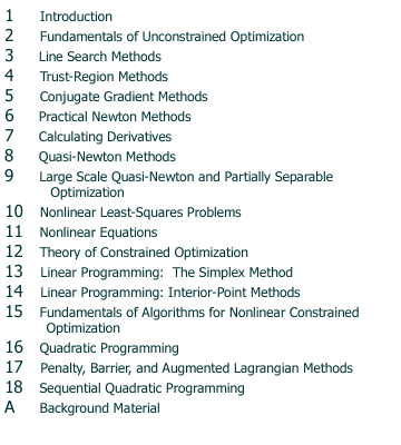
    COURSE TOPICS OUTLINE - C &O 466/666

    We will choose topics from the text. The complete list is included for now.


    Background Material Chapter Fifteen Chapter Fourteen Chapter Thirteen Chapter Twelve Chapter Eleven Chapter Ten Chapter Nine Chapter Eight Chapter Seven Chapter Six Chapter Five Chapter Four Chapter Three Chapter Two Chapter Eighteen Chapter Seventeen Chapter Sixteen Chapter One


    HOMEWORK LIST- C &O 466/666

    1. Homework #1 (Unconstrained Optimization)
      Due: Tuesday January 14, 2003 (at start of class)
      Reading
      Problems
      • Go to the NEOS Solvers web page. Use the unconstrained optimization package CGplus to solve the extended Rosenbrock function (see e.g. page 248 in the text or the sample submission for CGplus) with n=26 variables, parameter values alpha=10 and alpha=100, and method=2 (Polak-Ribiere).
        Then solve the problem using the unconstrained optimization package NMTR.
        Hand in (or email in) a copy of the outputs you get by email. In each case, point out the solution and the optimal value.
      • Pages 30-31, Problems 2.1, 2.3, 2.9, 2.10.
    2. Homework #2 (Unconstrained Optimization)
      Due: Thursday January 23, 2003 (at start of class)
      Reading Problems
      1. MATLAB
        1. Matlab appears to be on all the Solaris systems in the undergrad and grad environments, e.g. pythagoras, hopper, hermite and magnus. (The path is:
          /.software/local/.admin/bins/bin/matlab
          You should also have an account on (the multiple processor machine) tuxor. The default should now be version matlab-6.5. If not you should try the path software/matlab-6.5/bin/matlab or use "setenv PATH `/bin/showpath matlab-6.5 current`")
          Enter the command matlab to start up the matlab session. Then enter
          help optim
          You will see a list of the optimization functions that are available with the optimization toolkit.
        2. Now try the command
          optdemo
          This will bring up a menu. You can try the four choices. The first choice is a tutorial. This demonstrates several of the optimization functions.
        3. The second choice in the optdemo is the minimization of the banana function or Rosenbrock's function. This is a classical example of a function with a narrow valley that exhibits ``very'' slow convergence for steepest descent type methods. Try out several methods to minimize this function.
          1. Submit contour and surface plots of the banana function for variable values between -8,+8 (Use the matlab commands: help plot; or: demo )
          2. How many function evaluations did the minimization take for: steepest descent; simplex search; Broyden-Fletcher-Golfarb-Shanno; Davidon-Fletcher-Powell; Levenberg-Marquardt? (Please specify the line search you used.)
        Note: You can modify the matlab programs. You can see what the matlab routines are doing by looking at the matlab m-files. To do this change directory using: cd /software; cd matlab; cd distribution; cd toolbox; cd optim. In particular, there is an m-file called bandemo.m.
      2. Pages 62-63, Problems 3.2, 3.3, 3.5
      3. Homework #3 (BFGS and Newton; and Line Search Techniques)
        Due: Tuesday February 4, 2003 (at start of class)
        Reading Problems
        1. MATLAB
          Solve problem 3.9 on page 63 of the text. But do not program the BFGS algorithm yourself but rather use the matlab function for BFGS, i.e. you can find this by running optdemo and using the information, e.g. lines like
          [x,fval,exitflag,output] = fminunc({f,GRAD},x,OPTIONS);
          Output the values to verify that they indeed stay positive.
          Note: You can modify the matlab programs. You can see what the matlab routines are doing by looking at the matlab m-files. To do this change directory using: cd /software; cd matlab; cd distribution; cd toolbox; cd optim. In particular, there is an m-file called bandemo.m.
        2. Page 97, Problem 4.1
        3. Get the matlab program with the values for m,n,A,b given in the mat file, data.mat (you must save this 'binary' file). Use the files to
          minimize g(x) = sumi=1m log( e [aiTx - bi] +e [-aiTx + bi] )
          using Newton's method with backtracking. Which line search conditions are being guaranteed in this matlab program? What happens if you change the backtracking to guarantee the Strong Wolfe Conditions?
          Compare the optimal value with the least squares solution min ||Ax-b||.
      4. Homework #4 (Conjugate Gradient Methods, Practical Newton Methods)
        Due: Thursday February 13, 2003 (at start of class)
        Reading
        • Chapters 5,6 in the text (pages 100-162)
        Problems
        1. Page 133, Problems 5.5,5.8.
        2. MATLAB
          Use the conjugate gradient algorithm in the matlab program cgtrust.m to find the minimum of the banana function from the initial points: (-2,-3), (0,0), (-1.9,2), (-1.9,20).
            (BEWARE: In cgtrust.m, the initial radius of the trust region is set as the norm of the initial guess x0. Since this is zero for the (0,0) case, a divide by zero message appears. Quick-Fix correction:
            Line 56 ...old version... trrad=norm(x0);
            New version .............. trrad=norm(x0)+0.0001; % i.e. Add a small value
          Provide the number of major iterations and the final point to four decimals. Explain the behaviour.
          You will need the files dirdero.m and README. (You can use the default parameter values to start.)
      5. Homework #5 (NLLS, Nonlinear Equations, Nonlinear Programming)
        Due: Tuesday February 25, 2003 (at start of class)
        Reading
        • Chapters 10,11,12 in the text (pages 250-358)
        Problems
        1. MATLAB (try to use matlab 6)
          1. Test out the data fitting demo. This is one of the command line demos in the optimization toolkit. The example demonstrates fitting a nonlinear function to a set of data. Provide the plots of the data points; then provide the plots, number of iterations, function evaluations, and norm of the residual of the fit when using the Gauss-Newton method (with mixed polynomial interpolation) and, also when using sequential quadratic programming. Include the algebraic form of the nonlinear function that is used.
        2. Problems from text:
          1. Page 274, Problem 10.4.
          2. Page 311, Problem 11.8.
          3. Page 358, Problems 12.1,12.2,12.5.
      6. Homework #6 (Constrained Nonlinear Programming and Convex Analysis)
        Due: Thursday March 20, 2003 (at start of class)
        Reading Problems
        1. Constraint Qualifications
          1. Consider the general NLP with both equality and inequality constraints. Define the tangent cones and the linearizing cones at a feasible point x. Then show that the tangent cone is a subset of the linearizing cone.
          2. Consider the NLP:
              miniminze f(x,y,z)= ex + e-y+z
              subject to:
                g1(x,y,z)= ex -1 <= 0
                g2(x,y,z)= e-y -1 <= 0
                g3(x,y,z)= (x -1)2 + y2 -1 <= 0
                g4(x,y,z)= x2+y2+e-z -1 <= 0
              1. Verify that the NLP is a convex program.
              2. Use the KKT conditions to test for optimality at the origin (0,0,0)T.
              3. Use the Pshenichnyi conditions to test for optimality at (0,0,0)T.
              4. Is there a contradiction between the two tests for optimality? Find the linearizing cone at (0,0,0)T. Then find a direction in the linearizing cone that is not a tangent direction and use this to explain the discrepency.
        2. MATLAB (try to use matlab 6)
          1. Use the constrained optimization function fmincon in the optimization toolbox to solve the above convex program (problem 1.2 above). Can you get high accuracy in the solution?
        3. Problems from text:
          1. Page 359, Problem 12.10
          2. Page 360, Problem 12.17
          3. Page 418, Problem 14.11
        4. Homework #7 (Sample Problems for Final Exam)
          Due: Do NOT Hand IN.
          Chapter 15: Problems 15.1
          Chapter 16: Problems 16.2, 16.3, 16.4, 16.11, 16.13
          Chapter 17: Problems 17.2, 17.3
          Chapter 18: Problems 18.1, Describe the Maratos Effect and one possible "fix" for SQP methods.


        Mail to: hwolkowicz@uwaterloo.ca
        (C) Copyright Henry Wolkowicz, 2003.
        , by Henry Wolkowicz