Caution: May Contain Stable Sets Posted on June 4, 2022
In this blog post, we'll talk about the container method and two seemingly unrelated applications of it. Section 1 explains what the container method is, Section 2 describes two applications of the container method, and Section 3 shows how the applications are actually related.
A lot of the content in Section 1 and Section 2 comes from the course on the container method taught in Spring 2020 by Jorn van der Pol at the University of Waterloo. Part of the content in Section 3 is related to my current research with Jorn van der Pol and Peter Nelson.
1. What is the container method?
Many problems (real world and math) can be expressed with graphs and can be solved by counting various objects in these graphs. In this instance, we are interested in counting objects that can be represented by stable sets in a graph. It turns out there are many problems which can be represented this way, so we would like a method to count the number of stable sets in certain graphs. The container method, first used by Kleitman and Winston, is such a method. We will use a version of the container method for graphs, but note that there are other versions for hypergraphs.
Before we get started, I'll mention that by "stable" sets, I mean independent sets in a graph, but since matroids will come up later, I'm calling these sets stable instead of independent. That is, a stable set is a set of vertices where no two are adjacent.
I'll also mention some notation that will be used. The graph $G$ induced on vertex set $X$, denoted $G[X]$, is the graph with vertex set $X$ where two vertices are adjacent if and only if they are adjacent in $G$. We denote the number of edges and vertices of a graph $G$ by $e(G)$ and $v(G)$, respectively. Recall that the number of elements in a set $A$ is denoted $|A|$. Lastly, the set $\{1,\dots,n\}$ is denoted $[n]$.
Overview
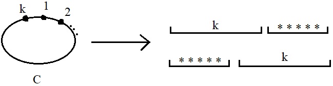
Every subset of a stable set is itself stable, so $2^{\text{ size of a largest stable set}}$ is a lower bound for the number of stable sets in a graph. It turns out this is often "almost" correct, up to a $(1+\text{o}(1))$ factor in the exponent, where o$(1)$ is a function of $v(G)$ that goes to 0 as $v(G)$ goes to infinity. The container method is a way to upper bound the number of stable sets by creating a bounded number of containers where each contains a bounded number of stable sets.
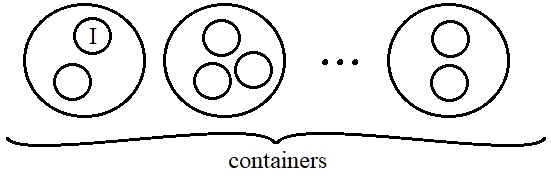
The figure above gives a visualization of the container method, although note that the stable sets are not all disjoint. I'll give a high level description of the theorem and then we'll get into the proof a little bit in the next subsection.
Container Theorem Sketch:
Let $G$ be a graph where the number of edges induced by a "large" set of vertices is "large".
Then there exists a collection $\mathcal{C}$ of containers (i.e. subsets of $V(G)$) such that:
- every stable set of $G$ is a subset of one of the containers in $\mathcal{C}$;
- the number of containers is "small"; and
- the size of each container is "small".
The idea is that the number of stable sets is bounded above by $\sum_{C\in \mathcal{C}}2^{|C|}$, which is at most $|\mathcal{C}|\cdot 2^{\max_{C\in \mathcal{C}} |C|}$. The theorem gives us an upper bound for this (based on the definition of "small").
Usually when we use the container method in a proof, we start with a corresponding lower bound for the number of stable sets in the applicable graph. We also usually prove a supersaturation lemma before using the container method. The goal of the supersaturation lemma is to show that the condition of the theorem holds. That is, it shows that the number of edges induced by a "large" set of vertices is "large".
Proof and Scythe Algorithm
To prove our container theorem, we construct the containers using a version of the Scythe Algorithm and then show that the constructed containers satisfy the desired definitions of "small". There are different versions of the Scythe algorithm for different applications, but they all have a similar flavour. Essentially, the algorithm takes in a stable set $I$ and outputs a subset (known as the fingerprint of $I$) and a superset (the container of $I$). I'll outline the algorithm more specifically below. Note that a maximum degree ordering of a set of vertices $A$ in a graph $G$ is a sequence $(v_1,\dots,v_{|A|})$ of the elements of $A$ where $v_i$ is the maximum degree vertex in $G[A-\{v_1\dots,v_{i-1}\}]$ with the smallest index.
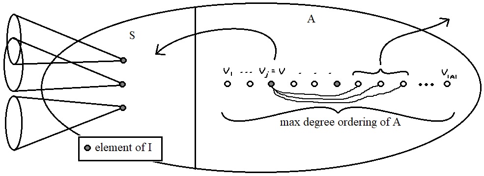
Scythe Algorithm
- Input: graph G, natural number $q$, stable set $I$ with $|I|\ge q$.
- Start with $S = \emptyset$ and $A = V(G)$.
- Repeat $q$ times:
- Let $v$ be the first element of $I$ in a maximum degree ordering of $A$.
- Move $v$ from $A$ to $S$.
- Remove the neighbours of $v$ from $A$.
- Output: $(S,A)$.
We can make a few claims about the sets $S$ and $A$; some follow easily and some require more proof. First, we claim that $S$ is the fingerprint of $I$ and $S\cup A$ (not $A$) is the container. In the algorithm, we only move vertices of $I$ into $S$, so clearly $S \subseteq I$. No neighbours of vertices in $I$ can be in $I$ themselves and the only vertices removed from $S\cup A$ are neighbours of those in $I$, so it follows that $I\subseteq S\cup A$.
We want the size of each container to be "small" and to do this we can try to bound the sizes of $S$ and $A$. Since the algorithm repeats $q$ times, we know that $|S| = q$. In order to bound $|A|$, we can figure out how many vertices are removed in each step. A lower bound for the number removed is determined using the placement of $v$ in the maximum degree ordering of $A$ and the fact that the number of edges in induced by a "large" set of vertices is "large". I'll skip the details, but suppose $R$ is found to be an upper bound for the size of each $A$. Then $|S\cup A|\le R + q$. That is: $$\text{size of each container } = |S| + |A| \le q+R.$$
We also want the number of containers to be "small", so we claim that for a graph $G$ with $N$ vertices, the number of outputs that the algorithm produces is relatively small. The first step is to show that if input $I$ produces output $(S,A)$, then input $S$ also produces output $(S,A)$. Have a look back at the algorithm and consider how it would run with input $I$ versus input $S$ to convince yourself that this is true. Now we know that the fingerprints determine the containers, so the number of containers is bounded above by the number of possible fingerprints, which is ${N\choose q}$ since $|S|=q$, plus the number of stable sets with size less than $q$, which is at most $\sum_{i=1}^{q-1} {N\choose i}$. That is: $$\# \text{ containers } \le \sum_{i=1}^q {N \choose i}.$$
Now we have shown that all parts of the Container Theorem hold for some definition of "small". The precise theorem is given in the next section.
Formal theorem and upper bound
Container Theorem
(Kohayakawa, Lee, Rödl, Samotij):
Let $q,N \in \mathbb{N}$, $R \in \mathbb{R}^+$, and $\beta \in [0,1]$ such that
$R \ge e^{-\beta q}N$.
Let $G$ be an $N$ vertex graph where
$$
e(G[U]) \ge \beta {|U| \choose 2} \text{ for every } U\in V(G) \text{ with at least }
R \text{ vertices.}
$$
There exists a collection $\mathcal{C}$ of containers such that:
- every stable set of $G$ is a subset of one of the containers in $\mathcal{C}$;
- the number of containers is at most $\sum_{i\le q} {N\choose i}$; and
- the size of each container is at most $R+q$.
Since each stable set is contained in one of the containers, we can bound the number of stable sets by $\sum_{C\in \mathcal{C}} (\#\text{ stable sets contained in } C)$. The number of stable sets contained in a container $C$ is at most the number of subsets of $C$, which is $2^{|C|}$. Now it follows that: $$ \# \text{ stable sets of } G \le \sum_{C\in \mathcal{C}} 2^{|C|} \le |\mathcal{C}|\cdot 2^{\max_{C\in \mathcal{C}} |C|}. $$
2. Seemingly unrelated applications
The following two problems demonstrate how the container method can be used. They both use a version of the method described above, but otherwise seem to be unrelated. It turns out these applications come up when looking at extensions and co-extensions of matroids that arise from cliques. In fact, both applications have come up in the research I'm doing now with Peter and Jorn. I'll get into this connection in Section 3 after I describe each problem and how the container method is applied.
Application 1: Antichains in the Boolean lattice
The Boolean lattice $\mathcal{P}([n])$ is the power set of $[n]$ partially ordered by $\subseteq$. For example, consider $\mathcal{P}([2])$, which is shown in the figure below. The elements of the Boolean lattice are $\emptyset,\{1\},\{2\},\{1,2\}$ and two sets are related if one contains the other as a subset.
![Hasse diagram of $\mathcal{P}([2])$.](Boolean_lattice_2.jpg)
A set $\mathcal{A}\in \mathcal{P}([n])$ is an \textbf{antichain} if its elements are pairwise unrelated. For example, $\{\{1\},\{2\}\}$ is an antichain in the example above.
![Hasse diagram of $\mathcal{P}([n])$.](Boolean_lattice_n.jpg)
Let's think about $\mathcal{P}([n])$ for general $n$ again.
Question: How many antichains are there?
By Sperner's theorem, we know the "middle" row is the largest antichain. That is, the largest antichain has size ${n \choose \lfloor n/2 \rfloor}$. Also, every subset of an antichain is itself an antichain, so the number of antichains is at least $2^{n\choose \lfloor n/2 \rfloor}$. It turns out the actual number is "almost" equivalent and we can use the container method to find the similar upper bound.
First, define a graph $G$ whose vertices are the elements of $\mathcal{P}([n])$ (i.e. subsets of $[n]$) and two sets are adjacent in $G$ if and only if one set contains the other. Notice that $G$ has $N=2^n$ vertices and its stable sets correspond to antichains in $\mathcal{P}([n])$.
Antichains of $\mathcal{P}([n])$ $\longleftrightarrow$ Stable sets of $G$
In order to apply the Container Theorem, we need to show that the number of edges induced by "large" sets of vertices is "large", so we prove a supersaturation lemma.
Supersaturation Lemma (Kleitman, 1968 **citation**):
If $U\subseteq V(G)$ and $|U|={n\choose n/2}+x$ for $x\ge 0$,
then $e(G[U]) \ge x(\lfloor n/2 \rfloor + 1)$.
Then we choose appropriate values for $R$, $q$, and $\beta$ so that the conditions of the theorem are satisfied. We choose $R = (1+\frac{1}{\sqrt{n}}){n\choose n/2}$, $q = \frac{\log n}{n}2^n$, and $\beta = \frac{n}{2^n}$ because reasons. Feel free to check that $R\ge e^{-\beta q}N$. Or you can take my word for it. Similarly, you can check that $e(U) \ge \beta {n\choose n/2}$ using the Supersaturation Lemma.
Using the values of $R$, $q$, and $\beta$, and the result of the Container Theorem we get: $$ |\mathcal{C}|\le \sum_{i\le q} {N\choose i} \le 2^{\text{o}(1){n \choose n/2}}, $$ and, for all $C\in \mathcal{C}$, $$ |C| \le R + q = (1+\text{o}(1)){n\choose n/2}. $$
As discussed earlier, the number of stable sets is at most $|\mathcal{C}| \cdot 2^{\max |C|}$. Therefore: $$ \# \text{ antichains } \le 2^{\text{o}(1){n \choose n/2}} \cdot 2^{(1+\text{o}(1)){n\choose n/2}}\\ = 2^{(1+\text{o}(1)){n\choose n/2}}. $$
Since $2^{{n\choose n/2}} \le \# \text{ antichains } \le 2^{(1+\text{o}(1)){n\choose n/2}}$, we find that the number of antichains in the Boolean lattice is $2^{(1+\text{o}(1)){n\choose n/2}}$. This was originally proved by Kleitman, although not by using this nice application of the container method. The details of this application are originally from Balogh, Treglown, and Wagner.
Application 2: Biased graphs
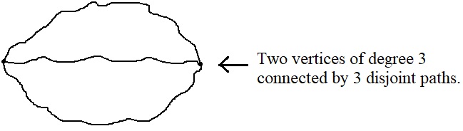
A biased graph is a pair $(G,\mathcal{B})$ where $G$ is a graph and $\mathcal{B}$ is a collection of cycles such that if two cycles $C,C'$ in $\mathcal{B}$ intersect in a non-empty path, then the third cycle in $C\cup C'$ is also in $\mathcal{B}$. Such a configuration of cycles is called a $\Theta$-subgraph and an example is shown in the figure below.
In other words, $\mathcal{B}$ satisfies the $\Theta$-property: for each $\Theta$-subgraph of $G$, either 0, 1, or 3 of its cycles are in $\mathcal{B}$. We call a biased graph $(G,\mathcal{B})$ scarce if $\mathcal{B}$ contains at most 1 cycle from each $\Theta$-subgraph of $G$.
If we're interested in the number of biased graphs, then we could start by considering the number of biased cliques. The number of graphs on $n$ vertices is $2^{{n\choose 2}}$ and each one is a subgraph of $K_n$, so the number of biased graphs is at most $2^{{n\choose 2}}$ times the number of biased cliques.
Question: How many biased cliques are there?
In the rest of this section, we'll answer this question by following Peter and Jorn's work in their paper "On the number of biased graphs".
Consider the set of Hamilton cycles of a clique $K_n$ and denote it by $\mathcal{B}$. At most one Hamilton cycle can be in a $\Theta$-subgraph, so $(K_n,\mathcal{B})$ is a biased clique. In fact, it is a scarce biased clique. Similarly, $(K_n,\mathcal{B}')$ is a (scarce) biased clique for each $\mathcal{B}'\subseteq \mathcal{B}$. The number of Hamilton cycles is $\frac{1}{2}(n-1)!$, so now we have a lower bound for the number of biased cliques.
$\#$ biased cliques $\ge 2^{\frac{1}{2}(n-1)!}$
As with antichains in the Boolean lattice, it turns out that this is "almost" correct, although it takes a bit more work prove it in this case. However, by using containers and a few other tricks, we can prove that the number of biased graphs is at most $2^{(1+\text{o}(1))\frac{1}{2}(n-1)!}$. The first step, however, is to prove the result for scarce biased cliques.
Define the Overlap Graph, denoted $\Omega_n$, to be the graph whose vertices are the cycles of $K_n$ where two cycles $C,C'$ are adjacent in $\Omega_n$ if and only if $C\cup C'$ is a $\Theta$-graph. Notice that the stable sets of $\Omega_n$ contain at most one cycle from each $\Theta$-subgraph of $K_n$, so they correspond to scarce biased cliques.
Scarce biased cliques $\longleftrightarrow$ Stable sets of $\Omega_n$
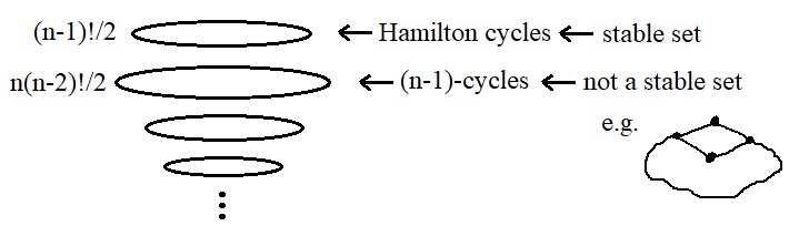
We can show that the unique maximum stable set in $\Omega_n$ is the set of Hamilton cycles of $K_n$ (which is done in Lemma 2.2 of Peter and Jorn's paper), but let's move on now to finding the upper bound for the number of stable sets.
First, we need to show that the number of edges induced by a "large" set of vertices is "large". That is, we need a supersaturation result.
Supersaturation Lemma (Peter and Jorn):
Let $\alpha \ge c/n$ where $c>0$ is some constant and let $\mathcal{B}\subseteq V(\Omega_n)$.
If $|\mathcal{B}| \ge (1+\alpha)\frac{1}{2}(n-1)!$, then
$e(\Omega[\mathcal{B}])\ge \frac{\alpha}{8}n!$.
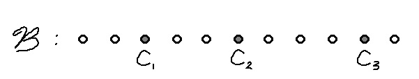
The proof of this Supersaturation Lemma has some tricky details, but the underlying idea is quite nice. The proof is by contradiction. We start by defining a mapping $\Phi$ from each cycle $C$ to permutations $\sigma$ of $[n]$ where either the first or the last $|C|$ elements of $\sigma$ describe a cyclic ordering of $C$. (This is shown in the figure below.)
Notice that for two cycles $C,C'$, we have $|\Phi(C)\cap \Phi(C')|\le 4$.
Let $\mathcal{B}_k$ be the cycles in $\mathcal{B}$ on $k$ vertices (i.e. $k$-cycles).
Then the idea is to find an upper bound for each $|\mathcal{B}_k|$ by bounding
$|\Phi(\mathcal{B}_k)|$ and the number of permutations in the image of two $k$-cycles,
using the knowledge that the intersection of the $\Phi$-images of two cycles is small.
This is where the details get complicated
(see the proof of Lemma 2.3 Peter and Jorn's paper),
but basically, using these upper bounds, we find that
$|\mathcal{B}| = \sum_{0\le k\le n-3} |\mathcal{B}_{n-k}|$ is too small, which gives the contradiction.
The next step is to apply the container method using this supersaturation result. Peter and Jorn prove a slightly different container theorem using a slightly different Scythe algorithm. One difference is that the loop in their algorithm repeats until $A$ is a certain size rather than exactly $q$ times. However, it works in a similar way and once all the details are worked out, we find that: $$ \# \text{ scarce biased cliques } \le 2^{(1+\text{o}(1))\frac{1}{2}(n-1)!} $$
We now need to show that the number of biased cliques is "almost" the same as the number of scarce biased cliques. The proof of this is quite clever, so I'll sketch it now.
Of the three cycles in a $\Theta$-subgraph of $K_n$, at least one has length at most $\frac{2}{3}(n+1)$. We call cycles of length at most $\frac{2}{3}(n+1)$ small cycles. The goal is to show that each biased clique can be determined by a scarce biased clique and a set of small cycles. We define a mapping $\psi: \{$biased cliques$\} \rightarrow \{$scarce biased cliques$\} \times \{$sets of small cycles$\}$ as follows. Let $(K_n,\mathcal{B})$ be a biased clique where the elements of $\mathcal{B}$ are partially ordered from smallest to largest.
For each triple of cycles $\{C_1,C_2,C_3\}\in \mathcal{B}$ that are in a $\Theta$-subgraph where $|C_1|\le |C_2|\le |C_3|$, remove $C_1$ and $C_3$ from $\mathcal{B}$, to obtain $\mathcal{B}'$. Notice that $(K_n,\mathcal{B}')$ is a scarce biased clique. Let $\mathcal{X}$ denote the set of small cycles in $\mathcal{B}$. Now, let $\psi((K_n,\mathcal{B})) = ((K_n,\mathcal{B}'),\mathcal{X})$.
Now we need to show that $\psi$ is an injection. Suppose it's not. That is, suppose two biased cliques with biases $\mathcal{B}_1$ and $\mathcal{B}_2$ map to the scarce biased clique with bias $\mathcal{B}$. Let $C$ be the smallest cycle in one bias, say $\mathcal{B}_1$, but not in the other, and not in $\mathcal{X}$. Since $\mathcal{B}_1$ and $\mathcal{B}_2$ both map to $\mathcal{B}$, we know $C$ gets deleted from $\mathcal{B}_1$; thus, $C$ is either $C_1$ or $C_3$ in a triple of cycles $\{C_1,C_2,C_3\}\in \mathcal{B}_1$ that make up a $\Theta$-subgraph. Since $C$ is not in $\mathcal{X}$, it is not a small cycle, and hence $C=C_3$. But then $\mathcal{B}_2$ contains $C_1$ and $C_2$, that is, two cycles from a $\Theta$-subgraph, which is a contradiction. Thus, we have proved that $\psi$ is a injection.
Since $\psi$ is a bijection, it follows that the number of biased cliques is at most the number of scarce biased cliques times the number of sets of small cycles. That is: $$ \# \text{ biased cliques } \le \# \text{ scarce biased cliques }\cdot 2^{\text{o}((n-1)!)} = 2^{(1+\text{o}(1))\frac{1}{2}(n-1)!}\cdot 2^{\text{o}((n-1)!))} = 2^{(1+\text{o}(1))\frac{1}{2}(n-1)!} $$ This completes the proof that the number of scarce biased cliques is "almost" the same at the number of biased cliques. Combining this with the lower bound from before we find: $$ \# \text{ biased cliques } = 2^{(1+\text{o}(1))\frac{1}{2}(n-1)!}. $$
Finally, recall that the number of biased graphs is at most $2^{{n\choose 2}}$ times the number of biased cliques. After a little bit of analysis depending on $n$ and the o$(1)$ term, we get: $$ \# \text{ biased graphs } = 2^{{n\choose 2}}\cdot 2^{(1+\text{o}(1))\frac{1}{2}(n-1)!} = 2^{(1+\text{o}(1))\frac{1}{2}(n-1)!}. $$
3. Connection to matroids
I'm going to go ahead and assume that you have some basic knowledge of matroids. If this is not the case, I recommend reading James Oxley's survey paper What is a matroid? Or, you could look at the first few slides of the talk I gave in the C&O Undergraduate Research Seminar on May 26, 2022.
Extensions
A matroid $N$ is a single-element extension of a matroid $M$ if $M\setminus e = N$ for some element $e\in E(M)$. That is, $N$ is the result of removing $e$ from $E(M)$ and removing all independent sets that contain $e$ from $\mathcal{I}$. For convenience, we'll refer to single-element extensions as simply extensions.
To me, matroids seem like mysterious objects. They generalize matrices and graphs, but there are many matroids beyond those related to matrices and graphs (i.e. non-representable matroids). In fact, almost all matroids are not representable, which Peter proved a few years ago. It is interesting to wonder how many matroids there are. The number of matroids on $n$ elements is only known for $n\le 9$ although there are upper and lower bounds for larger $n$. These bounds indicate that the number of matroids on $n$ elements is doubly exponential in $n$. One way to approach enumerating all matroids on $n$ elements is to consider the number of ways to "add" an element to a matroid. I think this is also an interesting question on its own. So now we're interested in attempting to find the number of extensions (or coextensions) of a matroid. This is a difficult question in general, so one idea is to start by considering extensions (and coextensions) of matroids that are dense, highly symmetric, and well understood. We'll consider extensions (and coextensions) of graphic matroids $M(K_n)$ that arise from cliques, which we'll call clique matroids.
Question: How many extensions of $M(K_n)$ are there?
In his 1965 paper, Crapo proves a collection of theorems which imply that there is a bijection between the linear subclasses of a matroid $M$ and the extensions of $M$. So now we are interested in determining the number of linear subclasses.
For clique matroids, a linear subclass is equivalent to a bias $\mathcal{B}\subseteq \{$unordered nontrivial bipartitions of $V(K_n)\}$ that satisfies the tripartition property: for each nontrivial tripartition $(A,B,C)$ of $V(K_n)$, $$ |\mathcal{B} \cap \{\{A\cup B,C\},\{A\cup C, B\},\{A, B\cup C\}\}| \in \{0,1,3\}. $$ We say the bias is scarce if this intersection is always at most 1.
At this point you might be wondering how this relates to the two applications discussed earlier. This definition looks similar to that of biased graphs, but where does the Boolean lattice come in? While this set up is very similar to biased graphs, they are actually related to coextensions, as we'll see in the coextensions subsection. It turns out that these scarce biases that represent extensions of $M(K_n)$ correspond to intersecting antichains in the Boolean lattice. An intersecting antichain is an antichain where no two elements are disjoint.
I'll give a bit of intuition for how these scarce biases are related to intersecting antichains. Consider a graph $\Pi_n$ whose vertices are the unordered nontrivial bipartitions of $V(K_n)$ where two vertices $\{A,B\},\{A',B'\}$ are adjacent if and only if $A\subseteq A'$ or $B \subseteq B'$ or $A\cap A' = \emptyset$ or $B\cap B' = \emptyset$. Notice that the stable sets in $\Pi_n$ correspond to scarce biases (which in turn correspond to extensions).
Since the bipartitions are unordered, we could instead consider ordered bipartitions where one element is fixed in, say, the first set. So choosing these biparitions is equivalent to choosing a subset of $[n-1]$. From here, it doesn't take too much effort to see that stable sets in $\Pi_n$ correspond to intersecting antichains in $\mathcal{P}([n-1])$.
The largest intersecting antichain in $\mathcal{P}([n-1])$ has size ${n-1\choose \lceil n/2 \rceil}= \frac{1}{2} {n \choose n/2}$, which gives a lower bound for the number of extensions of $M(K_n)$: $$ \# \text{ extensions of } M(K_n) \ge 2^{\frac{1}{2} {n \choose n/2}}. $$
The number of intersecting antichains is clearly less than the number of antichains, so by the final result in the antichains subsection: $$ \# \text{ scarce biases } \le 2^{(1+\text{o}(1)){n-1\choose (n-1)/2}} = 2^{(1+\text{o}(1))\frac{1}{2}{n\choose n/2}}. $$
Finally, we can use a lemma very similar to the one used to show that the number of scarce biased graphs is "almost" the same as the number of biased graphs to show that, in this setting, the number of scarce biases is "almost" the same as the number of biases. This gives us our final result: $$ \# \text{ extensions of } M(K_n) = 2^{(1+\text{o}(1))\frac{1}{2}{n\choose n/2}}. $$
Coextensions
A matroid $N$ is a single-element coextension of a matroid $M$ if $M/e = N$ for some element $e\in E(M)$. For convenience, we'll refer to single-element coextensions as simply coextensions.
Question: How many coextensions of $M(K_n)$ are there?
We can use Crapo's equivalence between extensions and linear subclasses here as well. For the duals of clique matroids, a linear subclass is equivalent to a bias $\mathcal{B}\subseteq \{$cycles of $K_n\}$ that satisfies the $\Theta$-property: for each $\Theta$-subgraph of $K_n$ with cycles $C_1,C_2,C_3$, $$ |\mathcal{B} \cap \{C_1,C_2,C_3\}| \in \{0,1,3\}. $$ Yup, you read that right, this is the definition of a biased clique! So now we know coextensions of $M(K_n)$ can be encoded by biased cliques.
In this case, all of the hard work was done when we analyzed biased graphs in the biased graphs subsection, so we immediately get: $$ \# \text{ coextensions of } M(K_n) = 2^{(1+\text{o}(1))\frac{1}{2}(n-1)!}. $$