Algorithms and Spectral Graph Theory
Table of Contents
- 1. About these notes
- 2. Linear Algebra notation & review
- 3. Matrices associated to graphs and their spectra
- 4. Cheeger's Inequality
- 5. Random walks
- 6. Electric networks
- 7. Maximum Cut and the Last Eigenvalue
- 8. Spectral Clustering
- 8.1. Introduction
- 8.2. Notations
- 8.3. Different ways to construct the similarity graph
- 8.4. Review of graph Laplacians
- 8.5. Spectral clustering algorithms
- 8.6. Graph cut point of view
- 8.7. Perturbation theory point of view
- 8.8. Justification by a slightly modified spectral algorithm
- 8.9. Practical details and issues
- 8.10. Conclusion
- 9. Bipartite Ramanujan Graphs and Interlacing Families
- 10. Improved Cheeger's Inequality
- 11. An Almost-Linear-Time Algorithm for Approximate Max Flow in Undirected Graphs, and its Multicommodity Generalizations
- 11.1. Resources
- 11.2. Problem definition and main result
- 11.3. Overview of the chapter
- 11.4. The Gradient Descent Method for general norms
- 11.5. Approximate Algorithm for the Maximum Flow Problem
- 11.5.1. Reformulation as Minimum Congestion Flow problem
- 11.5.2. Reformulation as a circulation problem
- 11.5.3. Reformulation as an unconstrained problem
- 11.5.4. Approximating \(\|\cdot\|_\infty\) by a smooth function
- 11.5.5. Solving the Maximum Flow Problem using the Gradient Descent Method
- 11.5.6. Constructing a projection matrix
\(\newcommand{\deff}{\mathrel{\mathop:}=}\newcommand{\rank}{\text{rank}}\newcommand{\trace}{\text{trace}}\newcommand{\onesv}{\mathbb{1}}\newcommand{\zerov}{\mathbb{0}}\newcommand{\E}{\mathbb{E}}\newcommand{\Span}{\text{span}}\newcommand{\R}{\mathbb{R}}\)
\(\newcommand{\extCur}{f^{\text{ext}}}\newcommand{\effResist}{R^{\text{eff}}}\)
\(\newcommand{\Cut}{\mathtt{cut}}\newcommand{\Uncut}{\mathtt{uncut}}\newcommand{\Deferred}{\mathtt{deferred}}\newcommand{\Cross}{\mathtt{cross}}\)
\(\newcommand{\norm}[1]{\|{#1}\|}\newcommand{\Norm}[1]{\left\|{#1}\right\|}\)
\(\newcommand{\sym}{\mathrm{sym}}\newcommand{\sgn}{\mathrm{sgn}}\newcommand{\fix}{\mathrm{fix}}\)
1 About these notes
These lecture notes are from course CO759 (Algorithms and Spectral Graph Theory) offered in Summer 2014. They are mostly based on lecture notes by Dan Spielman and/or Lap Chi Lau. The notes and illustrations where mostly prepared by Fidel Barrera-Cruz. Chapters 8, 9 and 10 were written by Hangmeng, Miaolan and Mehdi respectively who were graduate students taking the course.
These notes are released under the terms of the GNU Free Documentation License.
2 Linear Algebra notation & review
2.1 Some general notation
\([n]=\{1,\dots,n\}\), where \(n\) is a positive integer.
matrix \(A \in \mathbb{R}^{n\times{n}}\), column vector \(x\in \mathbb{R}^n\), then row vector is \(x^T\)
\(a_{i,j}\) : \((i,j)\)-th entry of \(A, \quad A_j\) : \(j\)-th column of \(A\),
\(\quad \widetilde{A}_{i,j}\) : matrix obtained from \(A\) by deleting \(i\)-th row and \(j\)-th column
2.2 Linear independence, span, basis, dimension, rank, \(\ldots\)
Linear (in)dependence: set of vectors \(\{ v_1,\dots,v_k \}\) is linearly independent if
\begin{equation} \nonumber c_1v_1+\dots+c_kv_k=0 \quad \Longrightarrow \quad c_i=0,\forall i \end{equation}otherwise the set is called linearly dependent.
Span of a set of vectors \(S\), denoted \(\text{span}(S)\), is the set of all linear combinations of the vectors in \(S\). If \(\text{span}(S)=\mathbb{R}^n\), then \(S\) is said to span \(\mathbb{R}^n\).
Basis of \(\mathbb{R}^n\) (or, of a vector space \(V\)) is a linearly independent set of vectors that spans \(\mathbb{R}^n\) (or, \(V\)).
Dimension of a vector space \(V\), denoted \(\text{dim}(V)\), is the size of a basis of \(V\).
For subspaces \(V_1\) and \(V_2\) (of a vector space \(V\)), the sum is \(\{ v_1 + v_2 : v_1\in V_1, v_2\in V_2 \}\) and it is denoted \(V_1 + V_2\). The intersection \(V_1\cap V_2 = \{ v : v\in V_1, v\in V_2 \}\) is a subspace, and we have \(V_1\cap V_2 \subseteq V_i \subseteq V_1+V_2,~i=1,2\).
(Dimension identity): Let \(V\) be a vector space (finite dimensional), and let \(V_1,V_2\) be subspaces of \(V\). Then
\begin{equation} \nonumber \text{dim}(V_1) + \text{dim}(V_2) = \text{dim} (V_1\cap V_2) + \text{dim} (V_1 + V_2). \end{equation}Nullspace (kernel) of \(A\): \(\text{nullsp}(A) = \{ x\in\mathbb{R}^n : Ax=0 \}\), and \(\text{null}(A)\) denotes the dimension of \(\text{nullsp}(A)\).
Range (image) of \(A\): \(\text{range}(A) = \{ Ax : x\in\mathbb{R}^n \}\), and its dimension is denoted \(\text{rank}(A)\); thus, \(\text{rank}(A) = \max\) no. of linearly independent columns of \(A\).
\begin{equation} \nonumber \text{rank}(A) + \text{null}(A) = n \end{equation}2.3 Determinant
\(\det(A) = \sum_{j=1}^n (-1)^{i+j} a_{i,j} \det( \widetilde{A}_{i,j} )\)
\(\det(A) = \sum_{\pi\in S^n} \text{sign}(\pi) \prod_{i=1}^n a_{i,\pi(i)}\), where \(\pi: [n] \rightarrow [n]\) is a permutation of \([n]\) (= index set of \(A\)), and \(\text{sign}(\pi) = (-1)^{\text{inv}(\pi)}\), where \(\text{inv}(\pi)\) denotes the number of inversions of \(\pi\), which is, \(\{(i,j):i\lt j\text{ and }\pi(i)>\pi(j)\}\)
\begin{align} \nonumber \det(A) \not=0 \quad &\text{ iff } \text{rank}(A)=n \notag \\ \det(A B) = \quad &\det(A) ~ \det(B) \notag \\ \text{rank}(A)=n \quad &\quad \Longrightarrow \quad A \text{ can be written as a product of elementary matrices} \end{align}2.4 Eigenvalues & eigenvectors
A nonzero-vector \(x\in\mathbb{R}^n\) is called an eigenvector of \(A\) if there exists a number \(\lambda\) s.t. \(Ax = \lambda x\) holds. We call \(\lambda\) an eigenvalue of \(A\).
\begin{equation} \nonumber Ax=\lambda x \text{ iff } (A-\lambda{I})x=0 \text{ iff } \text{null}(A-\lambda{I})\not= 0 \text{ iff } \text{rank}(A-\lambda{I})\lt n \text{ iff } \det(A-\lambda{I})=0 \end{equation}\(\det(A-\lambda{I})\) is a polynomial of \(\lambda\) of degree \(n\), called the characteristic polynomial of \(A\); each root is an eigenvalue. Thus, \(\det(A-\lambda{I}) = \prod_{i=1}^n (\lambda - \lambda_i)\), where \(\lambda_1,\dots,\lambda_n\) are the roots of the characteristic polynomial; so \(\lambda_1,\dots,\lambda_n\) are the eigenvalues of \(A\). If one of these roots \(\lambda_i\) appears \(k\) times, then we say that \(\lambda_i\) is an eigenvalue of multiplicity \(k\).
For a fixed eigenvalue \(\lambda\), any non-zero vector in \(\text{nullsp}(A-\lambda{I})\) is an eigenvector.
All real symmetric matrices have real eigenvalues (follows from Spectral theorem).
Geometric view: an eigenvector is a direction that is fixed (up to scaling) by the linear transform defined by \(A\)
Eigenspace: for an eigenvalue \(\lambda\), we call \(\text{nullsp}(A-\lambda{I})\) the eigenspace of \(\lambda\). We have: \(\text{null}(A-\lambda{I})\) is the geometric multiplicity of \(\lambda\).
2.5 Inner products, norm, orthonormal basis
Inner product of vectors \(u, v \in \mathbb{R}^n\), namely, \(\sum_{j=1}^n u_j v_j\) is denoted by \(\langle u,v\rangle\) (or by \(u\cdot{v}\))
Norm (or, length) of a vector \(v\) is \(\Vert v\Vert = \sqrt{\langle v,v\rangle}\)
Orthogonal (or, perpendicular) vectors \(u,v\): \(\langle u,v\rangle=0\)
Set of vectors \(\{v_1,\dots,v_n\}\) is orthogonal if \(\langle v_i,v_j\rangle=0,~ \forall i\neq{j}\)
Set of vectors \(\{v_1,\dots,v_n\}\) is orthonormal if it is orthogonal, and \(\Vert v_i\Vert=1, \forall i\)
Given any basis, we can construct an orthogonal basis by the Gram-Schmidt procedure: Given a basis \(B=\{w_1,\dots,w_k\}\), define the orthogonal basis \(B' = \{v_1,\dots,v_k\}\) by \(v_k = w_k - \sum_{j=1}^k \frac{ \langle w_k,v_j\rangle }{\Vert v_j\Vert} \; v_j,~\forall k: 2\le k\le n\) (and, \(v_1=w_1\)).
Then \(B''=\{ v_1/\Vert v_1\Vert, \dots, v_n/\Vert v_n\Vert \}\) is an orthonormal basis.
If \(B\) is a matrix whose columns form an orthonormal basis, then \(B^T B = I\) and hence the inverse of \(B\), denoted \(B^{-1}\), is equal to \(B^T\).
2.5.1 Cauchy-Schwarz Inequality
For vectors \(v,w \in\mathbb{R}^n\) we have
\begin{equation} \nonumber \vert\langle v,w\rangle\vert \leq \Vert v\Vert ~~ \Vert w\Vert, \end{equation}thus,
\begin{equation} \nonumber (\sum_{i=1}^{n} v_{i} w_{i}) ^2 \leq (\sum_{i=1}^{n} v_{i}^{2}) (\sum_{i=1}^{n} w_{i}^{2}) \end{equation}2.6 Spectral theorem
Let \(A\) be a real symmetric matrix. Then there exists an orthonormal basis of eigenvectors of \(A\) and the corresponding eigenvalues are real.
- Prove that all the eigenvalues of \(A\) are real.
- Find an eigenvalue \(\alpha_{n}\) and an eigenvector \(v_{n}\) of \(A\), and an orthonormal basis \(\mathcal{R}=\{u_{1},\ldots,u_{n-1}\}\) of the orthogonal complement of \(\Span(v_{n})\).
- Consider the matrix \(R\) having as columns the elements of \(\mathcal{R}\) and construct the \((n-1)\times (n-1)\) symmetric matrix \(B\) that has as entries the coefficients to obtain the vectors \(Au_{i}\) as a linear combination of elements in \(\mathcal{R}\).
- Inductively obtain the orthonormal basis of eigenvectors for \(B\), \(v_{1}'\ldots,v_{n-1}'\).
- The orthonormal basis of eigenvectors of \(A\) is obtained by normalizing the orthogonal basis of eigenvectors of \(A\) \(Rv_{1}',\ldots,Rv_{n-1}',v_{n}\).
We begin by showing that all the eigenvalues of \(A\) are real and then we proceed to show how to find the orthonormal basis of eigenvectors of \(A\) by induction.
Consider the polynomial \(p(\lambda)=\det(A-\lambda I)\). This polynomial has \(n\) roots, some may be complex. Let us begin by showing that all roots are real.
If \(u\) and \(v\) are eigenvectors of \(A\) associated to different eigenvalues, say \(\lambda_{u}\) and \(\lambda_{v}\) respectively, then \(u\) and \(v\) are orthogonal.
We have that \(\lambda_{v}u^{\intercal}v= u^{\intercal}(Av)=u^{\intercal}Av=(Au)^{\intercal}v=\lambda_{u}u^{\intercal}v\). Therefore \((\lambda_{v}-\lambda_{u})u^{\intercal}v=0\), and since \(\lambda_{v}\neq \lambda_{u}\) it follows that \(u^{\intercal}v=0\).
Now, let \(\lambda\) be a root of \(p\) and let \(v\) be an eigenvector associated to \(\lambda\). Then \(Av=\lambda v\). Taking complex conjugate on bot sides yields \(A\bar{v}=\bar{\lambda}\bar{v}\). So \(\bar{v}\) is an eigenvector of \(A\) with eigenvalue \(\bar{\lambda}\). Since \(v\neq 0\) we have that \(v^{\intercal}\bar{v}>0\). Thus by the previous claim it follows that the associated eigenvalues must be equal, that is, \(\lambda=\bar{\lambda}\). Therefore \(\lambda\in \mathbb{R}\).
We now know all eigenvalues of \(A\) are real. Let \(\alpha_{n}\) be one such eigenvalue. Before constructing the orthonormal basis of eigenvectors let us prove the following claim.
If \(U\) is an \(A\)-invariant subspace, then \(U^{\perp}\) is also an \(A\)-invariant subspace.
Let \(v\in U^{\perp}\) and \(u\in U\). Then \(u^{\intercal}(Av)=(Au)^{\intercal}v=(u')^{\intercal}v=0\). Thus \(Av\) is orthogonal to any \(u\in U\) and so \(Av\in U^{\perp}\), as desired.
Now, let \(v_{n}\) be an eigenvector associated to the eigenvalue \(\alpha_{n}\) and let \(U_{n}=\text{span}(v_{n})\). Observe that \(U_{n}\) is \(A\)-invariant. By the previous claim it follows that \(U_{n}^{\perp}\) is also \(A\)-invariant. Let \(u_{1},\ldots,u_{n-1}\) be an orthonormal basis of \(U_{n}^{\perp}\) and let \(R=[u_{1} \dots u_{n-1}]\). Then \(AR=[Au_{1} \dots Au_{n-1}]\), and since \(U_{n}^{\perp}\) is \(A\)-invariant we have that \(Au_{i}=\sum_{j\in [n-1]}b_{j,i}u_{j}\). So
\begin{equation} \nonumber AR=R \left[\begin{array}{rrrr} b_{1,1} & b_{1,2} & \dots & b_{1,n-1} \\ b_{2,1} & b_{2,2} &\dots & b_{2,n-1} \\ \vdots & \vdots & & \vdots\\ b_{n-1,1} & b_{n-1,2} & \dots & b_{n-1,n-1} \end{array}\right]= RB. \end{equation}Multiplying both sides by \(R^{T}\) and using the fact that \(u_{1},\ldots,u_{n-1}\) is an orthonormal basis we obtain \(R^{\intercal}AR=B\).
We claim that \(B\) is a symmetric matrix. Indeed since,
\begin{equation} \nonumber \begin{split} B_{i,j}&=u_{i}^{\intercal}Au_{j}\\ &=(Au_{j})^{\intercal}u_{i}\\ &=u_{j}^{\intercal}Au_{i}\\ &= B_{j,i}. \end{split} \end{equation}Thus \(B\) is an \((n-1)\times (n-1)\) real symmetric matrix. By induction hypothesis we have that \(B\) admits an orthonormal basis of eigenvectors \(v_{1}',\ldots,v_{n-1}'\) associated to eigenvalues \(\beta_{1},\ldots,\beta_{n-1}\). In particular \(Bv_{i}'=\beta_{i}v_{i}'\), which implies that \(R^{\intercal}ARv_{i}'=\beta_{i}v_{i}'\), or \(A(Rv_{i}')=\beta_{i}(R v_{i}')\). That is \(v_{i}\mathrel{\mathop:}=Rv_{i}'\) is an eigenvector of \(A\) with associated eigenvalue \(\beta_{i}\). Note that \(v_{n}\neq v_{i}\) for \(1\leq i\leq n-1\) since \(v_{i}\in U_{n}^{\perp}\) by the previous claim. Therefore \(\mathcal{B}=\{v_{1},\ldots,v_{n} \}\) is an orthogonal basis of eigenvectors of \(A\). The desired orthonormal basis can now be obtained by normalizing \(\mathcal{B}\).
Application: Power of matrix Let \(L\) be a matrix whose columns form an orthonormal basis of eigenvectors of \(A\). Then \(AL = LD\), where \(D\) is the diagonal matrix of eigenvalues. Thus, \(A = LDL^{-1} = LDL^T\).
We may compute the power \(A^k\) by multiplying the above \(k\) times to get \((LDL^T) (LDL^T) \dots (LDL^T) = L D^k L^T\). Note that \(D^k\) is easily computed: replace each entry \(\alpha\) of \(D\) by its power \(\alpha^k\).
Application: Eigen decomposition
Let \(\{v_1,\dots,v_n\}\) be an orthonormal basis of eigenvectors.
It can be seen that \(I = v_1v_1^T + v_2v_2^T + \dots + v_nv_n^T\).
Hence, we have \(Ax = A (v_1v_1^T + v_2v_2^T + \dots + v_nv_n^T) x = ( \lambda_1 v_1v_1^T + \lambda_2 v_2v_2^T + \dots + \lambda_n v_nv_n^T ) x\). Thus, \(A = \lambda_1 v_1v_1^T + \lambda_2 v_2v_2^T + \dots + \lambda_n v_nv_n^T\).
Assume \(\lambda_i\neq 0, \forall i\). Then we have, \(A^{-1} = \frac{1}{\lambda_1} v_1v_1^T + \frac{1}{\lambda_2} v_2v_2^T + \dots + \frac{1}{\lambda_n} v_nv_n^T\) because
\begin{equation} \nonumber \begin{split} ( \lambda_1 v_1v_1^T + \lambda_2 v_2v_2^T + \dots + \lambda_n v_nv_n^T ) ( \frac{1}{\lambda_1} v_1v_1^T + \frac{1}{\lambda_2} v_2v_2^T + \dots + \frac{1}{\lambda_n} v_nv_n^T ) &= (v_1v_1^T + v_2v_2^T + \dots + v_nv_n^T)\\ &= I. \end{split} \end{equation}2.7 Useful & Simple Inequalities
The following inequalities are useful; most of them are simple.
- For two real numbers \(\alpha, \beta\), we have \((\alpha + \beta)^2 \le 2 (\alpha ^2 + \beta ^2)\).
- For two integers \(\alpha, \beta \in \{-1,0,+1\}\), we have \((\alpha + \beta)^2 \le 2 |\alpha + \beta|\).
- Let \(\alpha_1,\beta_1\), \(\alpha_2,\beta_2\), …, \(\alpha_k,\beta_k\), be \(k\) pairs of nonnegative real numbers. Then we have
- Let \(x\in\mathbb{R}^{n}\) satisfy \(x \perp \mathbf{1}\) (thus, \(\sum_i x_i=0\)). Then \(\sum_{i\lt j} (x_i-x_j)^2 = n \sum_i x_i^2\).
2.8 References
This parts of the notes closely follows the expositions by Lau (week 1 and [[][]).
3 Matrices associated to graphs and their spectra
3.1 Matrices associated to graphs
Given a graph \(G\), there are several matrices we can associate to \(G\). Before stating them let us define \(D=\text{diag}(d_{1},\ldots,d_{n})\), where \(d_{i}\) denotes the degree of vertex \(i\). We can associate the following matrices to \(G\).
- The adjacency matrix \(A\). This is an \(n\times n\) \(01\)-matrix. The \(i,j\)-entry of \(A\), \(A_{i,j}\) is \(1\) if \(ij\in E\) and \(0\) otherwise.
- The normalized adjacency matrix \(\mathcal{A}\). This matrix is defined to be \(\mathcal{A}\deff D^{-1/2}AD^{-1/2}\).
- The Laplacian matrix \(L\). Here \(L\deff D-A\).
- The normalized Laplacian matrix \(\mathcal{L}\). This \(n\times n\) matrix is defined as \(\mathcal{L}\deff D^{-1/2}LD^{-1/2}=I-\mathcal{A}\).
Recall that the trace of a matrix \(M\) is defined to be the sum of its diagonal entries, that is, \(\trace(M)=\sum_{i=1}^{n}M_{i,i}\).
Let \(M\) be an \(n\times n\) matrix with eigenvalues \(\mu_{1},\ldots,\mu_{n}\). Then \(\trace(M)=\sum_{i=1}^{n}\mu_{i}\).
3.2 Spectra of the adjacency matrices of \(K_n\) and \(K_{m,n}\)
Let us begin by determining the spectrum of the adjacency matrix \(A\) for a couple of very specific kinds of graphs.
- Let \(G=K_{n}\), that is, let \(G\) be the complete graph on \(n\) vertices. In this case we have that \(A=J-I\), where \(J\) is the \(n\times n\) matrix with all entries equal to 1. Observe that \(I\) has \(1\) as an eigenvalue with multiplicity \(n\). Now, since \(J\) has rank \(1\), it follows that \(0\) is an eigenvalue of \(J\) with multiplicity \(n-1\). Finally, observe that \(\onesv\) is an eigenvector of \(J\) with eigenvalue \(n\). Thus \(J\) has as eigenvalues \(0\) with multiplicity \(n-1\) and \(n\) with multiplicity \(1\). This implies that \(A\) has eigenvalues \(-1\) with multiplicity \(n-1\) and \(n-1\) with multiplicity \(1\).
- Let \(G=K_{m,n}\), the complete bipartite graph with partite
sets \(X\) and \(Y\). We may assume, without loss of generality, that
\(X=\{1,\ldots,m\}\) and \(Y=\{m+1,\ldots,m+n\}\). Thus
\begin{equation*}
A= \left[\begin{array}{rr}
0& J_{m,n} \\
J_{m,n}^{\intercal} & 0 \\
\end{array}\right],
\end{equation*}
where \(J_{m,n}\) is the \(m\times n\) all ones matrix. Note that
\(\rank(A)=0\), so \(0\) is an eigenvalue of \(A\) with multiplicity \(n-2\). Now, since the trace of \(A\) is \(0\), we have that the sum of the eigenvalues of \(A\) is \(0\). Thus the two remaining eigenvalues, call them \(\alpha_{1}\) and \(\alpha_{2}\), must satisfy \(\alpha_{1}=-\alpha_{2}\). So far we know that
\begin{equation*} \begin{split} \det(A-\alpha I) &= \alpha^{m+n-2}(\alpha-\alpha_{1})(\alpha-\alpha_{2})\\ &= \alpha^{m+n-2}(\alpha^{2}-\alpha_{1}^{2})\\ &= \alpha^{m+n}-\alpha_{1}^{2}\alpha^{m+n-2}\\ &= \alpha^{m+n}-x\alpha^{m+n-2}, \end{split} \end{equation*}where \(x=\alpha_{1}^{2}\). By computing the determinant of \(\alpha I-A\) we can observe that for each edge of \(G\) there is exactly one \(\alpha^{m+n-2}\). Since there are precisely \(mn\) such terms this implies that the coefficient of \(\alpha^{m+n-2}\) is \(mn\), that is \(x=mn\). Therefore \(\alpha_{1}=\sqrt{mn}\) and \(\alpha_{2}=-\sqrt{mn}\). Thus \(K_{m,n}\) has eigenvalues \(\sqrt{mn}\) and \(-\sqrt{mn}\) with multiplicity \(1\), and \(0\) with multiplicity \(m+n-2\).
3.3 A characterization of bipartiteness
Recall that the spectrum of the adjacency matrix of the complete bipartite graph \(K_{m,n}\) is symmetric about \(0\). In fact, as we will see in the following result, this property charecterizes bipartite graphs.
Let \(G\) be a graph. Then \(G\) is bipartite if and only if for any nonzero eigenvalue \(\alpha\) of \(A\), \(-\alpha\) is also an eigenvalue of \(A\).
Let us begin by assuming \(G\) is bipartite, with partite sets \(X\) and \(Y\). Without loss of generality we may assume that \(X=\{1,\ldots,k\}\) and \(Y=\{k+1,\ldots,n\}\). Thus
\begin{equation*} A= \left[\begin{array}{rr} 0& B \\ B^{\intercal} & 0 \\ \end{array}\right], \end{equation*}where \(B\) is some \(k\times n-k\) \(01\)-matrix. Let \(\alpha\) be an eigenvalue of \(A\) with eigenvector \(z=[x,y]^{\intercal}\). Then
\begin{equation*} \left[\begin{array}{r} By \\ B^{\intercal}x \\ \end{array}\right] = \left[\begin{array}{rr} 0& B \\ B^{\intercal} & 0 \\ \end{array}\right] \left[\begin{array}{r} x \\ y \\ \end{array}\right] \\ = Az\\ = \alpha z\\ = \left[\begin{array}{r} \alpha x \\ \alpha y \\ \end{array}\right]. \end{equation*}So \(By=\lambda x\) and \(B^{\intercal}x=\lambda y\). We now have that
\begin{equation*} \left[\begin{array}{rr} 0& B \\ B^{\intercal} & 0 \\ \end{array}\right] \left[\begin{array}{r} x \\ -y \\ \end{array}\right] = \left[\begin{array}{r} -By \\ B^{\intercal}x \\ \end{array}\right] = -\alpha \left[\begin{array}{r} x \\ -y \\ \end{array}\right] \end{equation*}So \([x,-y]^{\intercal}\) is an eigenvector of \(A\) with eigenvalue \(-\alpha\). Note that \(k\) linearly independent eigenvectors associated to \(\lambda\) would yield \(k\) linearly independent eigenvectors associated to \(-\lambda\).
Let us now prove the converse implication. It can be shown by induction that the \(i,j\) entry of \(A^{k}\) is equal to the number of \(ij\)-walks of length \(k\) in \(G\). This implies that the entries of \(A^{k}\) are nonnegative. In particular \(A^{k}_{i,i}\geq 0\) for all \(i\in [n]\). We use this observation together with the fact that nonzero eigenvalues come in positive negative pairs to show that \(G\) is bipartite.
Note that if \(\alpha_{1},\ldots,\alpha_{n}\) are the eigenvalues of \(A\), then \(\alpha_{i}^{k},\ldots,\alpha_{n}^{k}\) are the eigenvalues of \(A^{k}\). THus, for odd \(k\) we have that \(\trace(A^{k})=\sum_{i\in [n]}\alpha_{i}^{k}=0\), and since \(A^{k}_{i,i}\geq 0\), it follows that \(A^{k}_{i,i}=0\) for all \(i\in [n]\). That is, \(G\) contains no \(ii\)-walks of odd length \(k\), in particular \(G\) contains no odd cycles. Therefore \(G\) is bipartite.
3.4 Positive semidefinite matrices and the Laplacian
Let us now turn our attention to the spectrum of the Laplacian matrix \(L\) of a graph \(G\). Recall that \(L\deff D-A\), where \(D\) is the diagonal matrix with \(D_{i,i}\) being the degree of vertex \(i\) and \(A\) is the adjacency matrix of \(G\).
Note that if we add the entries of a row in \(L\) we obtain \(0\), since \(d_{i}\) will cancel out with the \(d_{i}\) \(-1\)'s that are off the diagonal in that row. This implies that \(L\onesv =\zerov\), or that \(\onesv\) is an eigenvector with eigenvalue \(0\). We will now see that \(0\) is the smallest eigenvalue of \(L\). Let \(e=ij\) and let \(b_{e}\) be the \(n\times 1\) column vector with entry \(i\) being \(1\), entry \(j\) being \(-1\) and \(0\) elsewhere. It is left as an exercise to the reader to show that if \(B=[b_{e_{1}}\dots b_{e_{m}}]\) is the \(n\times m\) matrix with columns given by the \(b_{e}\) vectors defined above, then \(L=B B^{\intercal}\).
We need to introduce one more concept and prove one more lemma before we are able to show that \(0\) is the smallest eigenvalue of \(L\).
A real symmetric matrix is said to be positive semidefinite if \(x^{\intercal}Mx\geq0\) for all \(x\in \R^{n}\).
Let \(M\) be a real symmetric matrix. The following are equivalent
- \(M\) is positive semidefinite.
- All the eigenvalues of \(M\) are nonnegative.
- \(M=BB^{\intercal}\) for some matrix \(B\).
We begin by making an observation for real symmetric matrices. Since \(M\) is symmetric, it is similar to a diagonal matrix \(S\) having the eigenvalues of \(M\) in its diagonal. Furthermore \(M=RSR^{\intercal}\) with the columns of \(R\) defining an orthonormal basis of eigenvectors of \(M\).
Let us show that 1 implies 2. Since \(M\) is positive semidefinite taking \(x=Re_{i}\), with \(e_{i}\) being the \(i\)-th standard basis vector, we obtain that
\begin{equation*} 0\leq x^{\intercal}Mx=(Re_{i})^{\intercal}MRe_{i}=e_{i}^{\intercal}Se_{i}=S_{i,i}. \end{equation*}So \(S_{i,i}\geq 0\) for all \(i\in [n]\).
Now, we show that 2 implies 3. Since all entries of \(S\) are nonnegative and since \(S\) is diagonal we have that
\begin{equation*} M=RSR^{\intercal}=RS^{1/2}S^{1/2}R^{\intercal}=(S^{1/2}R^{\intercal})^{\intercal}S^{1/2}R^{\intercal}=B^{\intercal}B, \end{equation*}as desired.
Finally let us show that 3 implies 1. If \(M=BB^{\intercal}\), then
\begin{equation*} x^{\intercal}Mx=x^{\intercal}BB^{\intercal}x=(B^{\intercal}x)^{\intercal}(B^{\intercal}x)=\Vert B^{\intercal} x\Vert^{2}\geq 0, \end{equation*}for all \(x\in \R^{n}\). Thus \(M\) is positive semidefinite.
3.5 Connectedness and the Laplacian matrix
We have established that \(0\) is the smallest eigenvalue of the Laplacian matrix of a graph. In the following result we explore the relation between the eigenvalue of the Laplacian \(0\) and the number of connected components of a graph.
A graph is connected if and only of \(0\) is an eigenvalue of \(L\) with multiplicity \(1\).
If \(G\) is not connected, then we can partition its vertex set into two sets \(S_{1}\) and \(S_{2}\) such that no edge has an endpoint in both \(S_{1}\) and \(S_{2}\). Suppose without loss of generality that \(S_{1}=\{1,\ldots,k\}\) and \(S_{2}=\{k+1,\ldots,n\}\). Let \(\chi_{S_{1}}=[\underbrace{1,\ldots,1}_{k},\underbrace{0,\ldots,0}_{n-k}]\) and let \(\chi_{S_{2}}=\onesv-\chi_{S_{1}}\). Observe that \(L\chi_{S_{1}}=L\chi_{S_{2}}=\zerov\), so \(\chi_{S_{1}}\) and \(\chi_{S_{2}}\) are eigenvectors of \(L\) associated to eigenvalue \(0\). Thus \(0\) has multiplicity at least two.
Now, suppose \(G\) is connected and consider \(x^{\intercal}Lx=\sum_{ij\in E}(x_{i}-x_{j})^{2}\geq0\). If \(x\) is an eigenvector associated to \(0\), then \(Lx=\zerov\), so \(x^{\intercal}Lx=0\). This implies \(x_{i}=x_{j}\) for every edge \(ij\). Since \(G\) is connected, the value for a given \(x_{j}\) propagates to all vertices of \(G\). Thus \(x=c\onesv\), that is, any eigenvector is a multiple of \(\onesv\). Therefore the eigenvalue \(0\) has multiplicity \(1\).
3.6 Courant-Fischer inequality
For a real symmetric matrix \(A\) we define the Rayleigh quotient
\begin{equation} \nonumber R(x)\mathrel{\mathop:} = \frac{x^{\intercal}Ax}{x^{\intercal}x} = \frac{\sum_{i,j}a_{i,j}x_{i}x_{j}}{\sum_{i}x_{i}^{2}}. \end{equation}Suppose \(A\) has eigenvalues \(\alpha_{1}\geq \alpha_{2}\geq \ldots \geq \alpha_{n}\) with corresponding orthonormal eigenvectors \(v_{1},\ldots,v_{n}\).
The largest eigenvalue of \(A\) can be expressed as
\begin{equation} \nonumber \alpha_{1}=\max_{x\neq 0}\,R(x). \end{equation}Let \(x\in\mathbb{R}^{n}\) with \(x\neq 0\), then \(x=a_{1}v_{1}+\dots+a_{n}v_{n}\). So
\begin{equation} \label{eq:precourant-numerator} \begin{split} x^{\intercal}Ax &= (a_{1}v_{1}+\dots+a_{n}v_{n})^{\intercal}A(a_{1}v_{1}+\dots+a_{n}v_{n})\\ &=\sum_{i\in[n]}a_{i}^{2}v_{i}^{\intercal}Av_{i}+2\sum_{i\neq j}a_{i}a_{j}v_{i}^{\intercal}Av_{j}\\ &=\sum_{i\in[n]}\alpha_{i}a_{i}^{2} \end{split} \end{equation}Note that \(x^{\intercal}x=(a_{1}v_{1}+\dots+a_{n}v_{n})^{\intercal}(a_{1}v_{1}+\dots+a_{n}v_{n})=\sum_{i\in[n]}a_{i}^{2}\).
Therefore
\begin{equation} \nonumber R(x)=\frac{\sum_{i\in[n]}\alpha_{i}a_{i}^{2}}{\sum_{i\in[n]}a_{i}^{2}}\leq \alpha_{1}\frac{\sum_{i\in[n]}a_{i}^{2}}{\sum_{i\in[n]}a_{i}^{2}}=\alpha_{1}. \end{equation}Thus \(R(x)\leq \alpha_{1}\) for all \(x\neq 0\) and taking \(x=v_{1}\) we obtain \(R(v_{1})=\alpha_{1}\) which concludes the proof.
Let \(T_{k}\) denote the orthogonal complement of the subspace spanned by \(v_{1},\ldots,v_{k-1}\), that is, \(T_{k}=\Span(v_{1},\ldots,v_{k-1})^{\perp}\). Then
\begin{equation} \nonumber \alpha_{k}=\max_{x\in T_{k}}R(x). \end{equation}Let \(x\in T_{k}\) and write \(x=a_{1}v_{1}+\dots +a_{n}v_{n}\). Note that \(x^{\intercal}v_{i}=a\Vert v_{i}\Vert^{2}=a_{i}\). Since \(x\in T_{k}\) it follows that \(a_{i}=x^{\intercal}v_{i}=0\) for \(1\leq i\leq k-1\). Thus \(x=a_{k}v_{k}+\dots+a_{n}v_{n}\).
Now \(x^{\intercal}Ax=\sum_{i=k}^{n}a_{i}^{2}\alpha_{i}\), by a similar reasoning as in \eqref{eq:precourant-numerator}. Also \(x^{\intercal}x=\sum_{i=k}^{n}a_{i}^{2}\). Therefore we have that
\begin{equation} \nonumber R(x)=\frac{\sum_{i=k}^{n}a_{i}^{2}\alpha_{i}}{\sum_{i=k}^{n}a_{i}^{2}}\leq \alpha_{k} \frac{\sum_{i=k}^{n}a_{i}^{2}}{\sum_{i=k}^{n}a_{i}^{2}} =\alpha_{k}. \end{equation}Thus \(R(x)\leq \alpha_{k}\) for all \(x\in T_{k}\) and taking \(x=v_{k}\) we obtain \(R(v_{k})=\alpha_{k}\), as desired.
Note that the previous result allows us to obtain \(\alpha_{k}\) provided we know \(T_{k}\). The following result, the Courant-Fischer Theorem, gives a characterization of \(\alpha_{k}\) that does not depend on knowing \(T_{k}\) and it can be used for providing bounds for the eigenvalues of a matrix.
For a real symmetric matrix \(A\) we have that the \(k\)-th largest eigenvalue \(\alpha_{k}\) is given by
\begin{equation} \nonumber \alpha_{k}=\max_{\substack{S\subseteq \R^{n}\\ \dim(S)=k}}\min_{x\in S}\, R(x) = \min_{\substack{S\subseteq \R^{n}\\ \dim(S)=n+k-1}} \max_{x\in S}\, R(x). \end{equation}We only prove the \(\max\)-\(\min\) relation, the \(\min\)-\(\max\) relation can be proved by a similar argument. Let \(S_{k}=\Span(v_{1},\ldots,v_{k})\) and let \(x\in S_{k}\). Write \(x=a_{1}v_{1}+\dots+a_{k}v_{k}\). Following a similar reasoning as in the proofs of the previous two lemmas we have that
\begin{equation} \nonumber R(x)= \frac{\sum_{i\in[k]}\alpha_{i}a_{i}^{2}}{\sum_{i\in[k]}a_{i}^{2}} \geq \alpha_{k}\frac{\sum_{i\in[k]}a_{i}^{2}}{\sum_{i\in[k]}a_{i}^{2}}=\alpha_{k}. \end{equation}So
\begin{equation} \nonumber \max_{\substack{S\subseteq \R^{n}\\ \dim(S)=k}}\min_{x\in S}\, R(x) \geq \min_{x\in S_{k}}\, R(x)\geq \alpha_{k}. \end{equation}Now, any \(k\) dimensional vector space \(S\) intersects the \(n-k+1\) dimensional vector space \(T_{k}=\Span(v_{k},\ldots,v_{n})\). By the previous lemma we have that \(\alpha_{k}=\max_{x\in T_{k}}\, R(x)\), therefore
\begin{equation} \nonumber \max_{\substack{S\subseteq \R^{n}\\ \dim(S)=k}}\min_{x\in S}\, R(x) \leq \max_{\substack{S\subseteq \R^{n}\\ \dim(S)=k}}\min_{x\in S\cap T_{k}}\, R(x) \leq \alpha_{k.} \end{equation}Putting the last two inequalities together yields the first part of the result.
4 Cheeger's Inequality
4.1 Cheeger's Inequality (Laplacian)
In this section we study Cheeger's inequality, which provides a bound on how well connected a graph is in terms of the second smallest eigenvalue of its Laplacian matrix.
We have previously seen that a graph \(G\) is disconnected if and only if its second smallest eigenvalue \(\lambda_{2}\) is \(0\). Informally, Cheeger's inequality states that the second smallest eigenvalue is close to \(0\) if and only if there is a sparse cut in \(G\). Let us now formalize this by introducing the concept of conductance.
A measure of connectedness of a graph \(G=(V,E)\) is its conductance. The conductance of a nonempty set \(S\subseteq V\) is defined to be
\begin{equation} \nonumber \frac{e(S,V-S)}{\min\{|V|,|V-S|\}}. \end{equation}The conductance of the graph \(G\), \(\Phi\), is defined to be the minimum of the conductances over all nonempty subsets of \(V\), in symbols
\begin{equation} \nonumber \Phi = \min_{\emptyset\neq S\subseteq V}\frac{e(S,V-S)}{\min\{|V|,|V-S|\}}. \end{equation}Let \(G=(V,E)\) be an undirected graph, and let \(\Phi = \min_{\emptyset\not=S\subsetneq{V}} \frac{e(S,V-S)}{\min \{ |S|, |V-S|\}}\) denote its conductance; also, let \(d_{\max}\) denote the maximum of the degree of the nodes. Let \(\lambda_2\) denote the second smallest eigenvalue of the Laplacian matrix \(L(G)\). Then,
\begin{equation} \nonumber \frac{\lambda_{2}}{2} \leq \Phi \leq \sqrt{2\lambda_{2}d_{\max}} \end{equation}(Follows Kelner's course notes for MIT:18.409:F2009)
Lowerbound (Easy):
Let \(S\subsetneq{V}\) (nonempty) denote a cut \((S,V-S)\) that defines \(\Phi\). We proceed by using the fact that \(|S|\cdot|V-S|\geq n/2\min\{|S|,|V-S|\}\) and then showing that the resulting quotient is at least as big as the minimum of all quotients when restricted to the vectors orthogonal to \(\mathbb{1}\), which by the Courant-Fischer inequality is precisely \(\lambda_{2}\).
Then
\begin{equation} \nonumber \begin{split} \Phi &= \frac{ e(S,V-S) }{\min\{|S|,|V-S|\}} \geq (n/2) \frac{ e(S,V-S) }{ |S| |V-S| } \\ &= (n/2) \frac{ \sum_{ij\in E} (x_i-x_j)^2 } { \sum_{i\lt j} (x_i-x_j)^2 } \qquad (\mbox{taking $x = \chi^{S}-\chi^{V-S}$}) \\ & \geq (n/2) \min_{x\in \mathbb{R}^n,\; x\perp\mathbf{1}} \frac{ \sum_{ij\in E} (x_i-x_j)^2 } { \sum_{i\lt j} (x_i-x_j)^2 } \\ &=~ (n/2) \min_{x\in \mathbb{R}^n,\; x\perp\mathbf{1}} \frac{ \sum_{ij\in E} (x_i-x_j)^2 } { n \sum_{i} x_i ^2 } \\ &=~ \frac12 \lambda_2. \end{split} \end{equation}Upperbound (NotEasy – follows Spielman~F98, Kelner~F09):
For a vector \(y\in\mathbb{R}^n\), define \(R(y) = \frac{ y^T L y }{ y^T y }\), the Rayleigh quotient of \(y\).
Goal: for any vector \(x \perp\mathbf{1}\), we have \(R(x) \geq \frac{\Phi^2}{ 2d_{\max} }\), in other words, \(\Phi \leq \sqrt{ 2 d_{\max} R(x) }\).
(Aside: Since \(\lambda_2 = \min_{x\in \mathbb{R}^n,\; x\perp\mathbf{1}} R(x)\), we will get \(\lambda_2 \geq \frac{\Phi^2}{ 2d_{\max} }\).)
We prove something stronger:
Index the nodes s.t. \(x_1 \le x_2 \dots \le x_n\).
Assume \(n\) is odd, and let \(m\) denote the "median index", \(m = (n+1)/2\).
Define the canonical cuts for \(i=1,\dots,n\) by \((S_i,\overline{S_i})\) where \(S_i\) is defined as follows: () if \(i\leq m\), then \(S_i = \{1,\dots,i\}\), otherwise () (so, \(i>m\)) \(S_i = \{ i, i+1, i+2, \dots, n \}\).
Then, for the ``best'' of the canonical cuts, we have \(\Phi \leq e(S_i,\overline{S_i})/|S_i| \leq \sqrt{ 2 d_{\max} R(x) }\).
Preprocess to split \(G\) into left-subgraph and right-subgraph with common node \(m\)
Define \(y = x - x_m \mathbf{1}\), thus \(y_i = x_i - x_m, \forall i\).
Claim: \(R(x) \geq R(y)\).
Proofsketch: For the numerators (top part) we have \(x^T L x = \sum_{ij\in E} (x_i-x_j)^2 = y^T L y\). For the denominators (bot part) we have \(x^T x \leq y^T y = (x - x_m \mathbf{1})^T (x - x_m \mathbf{1}) = x^Tx + n x_m^2 - 2x_m (x^T\mathbf{1}) = x^Tx + n x_m^2\) (since \(x\perp\mathbf{1}\)).
Next, transform \(G\) to \(G^{new} = (V, E^{new})\) by replacing each edge \(ij\) in the canonical cut \((S_m,\overline{S_m})\) by the two edges \(im, mj\); i.e., subdivide each edge in this cut by a new node and identify all the new nodes with \(m\); both \(V\) and \(y\) stay the same.
Claim: \(R(y, G) \geq R(y, G^{new})\).
Proofsketch: Consider the contributions from a transformed edge \(ij\) to the numerators (top part); we have, \((y_j - y_i)^2 = ((y_j - y_m) + (y_m - y_i))^2 \geq (y_j - y_m)^2 + (y_m - y_i)^2\).
Let the left subgraph \(G_L = (V_L, E_L)\) be the subgraph induced by \(V_L = \{1,\dots,m\}\).
Let the right subgraph \(G_R = (V_R, E_R)\) be the subgraph induced by \(V_R = \{m,m+1,\dots,n\}\).
Since \(y_m=0\) (this explains the choice of \(y\)), we have (for numerator) \(y^T L(G^{new}) y = \sum_{ij\in E_L} (y_i-y_j)^2 ~~+~~ \sum_{ij\in E_R} (y_i-y_j)^2\), and (for denominator) \(y^T y = \sum_i y_i^2 = (\sum_{i\in V_L} y_i^2) + (\sum_{i\in V_R} y_i^2)\).
Thus
\begin{equation} \nonumber \begin{split} R(y, G^{new}) &= \frac{ y^T L(G^{new}) y }{y^T y}\\ &=\frac{ \sum_{ij\in E_L} (y_i-y_j)^2 + \sum_{ij\in E_R} (y_i-y_j)^2 } { \sum_{i\in V_L} y_i^2 + \sum_{i\in V_R} y_i^2 }\\ &\geq \min \{ \frac{ \sum_{ij\in E_L} (y_i-y_j)^2 }{\sum_{i\in V_L} y_i^2}, \frac{ \sum_{ij\in E_R} (y_i-y_j)^2 }{\sum_{i\in V_R} y_i^2} \} \\ &= \min\{ R(y, G_L), R(y, G_R) \}. \end{split} \end{equation}We claim that each of \(R(y, G_L)\) and \(R(y, G_R)\) is \(\geq \frac{\Phi^2 }{2d_{\max}}\).
Plan for this part:
Key Lemma (Kelner):
Consider \(z \in \mathbb{R}^{V_L}_{-}\) and index the nodes s.t. \(z_1 \le z_2 \le \dots \le z_m = 0\). Then \(\sum_{ij\in E_L} |z_i - z_j| \ge \Phi(G) \sum_i |z_i|\).
Scale \(y\) s.t. \(\sum_{i\in V_L} y_i^2 = 1\).
Apply Cauchy-Schwarz inequality to get
\begin{equation} \nonumber \sum_{ij\in E_L} |y_i^2 - y_j^2| ~~=~~ \sum_{ij\in E_L} |y_i - y_j|~~|y_i + y_j| ~~\leq~~ \sqrt{\sum_{ij\in E_L} (y_i-y_j)^2} ~~ \sqrt{\sum_{ij\in E_L} (y_i+y_j)^2}. \end{equation}Thus
\begin{equation} \nonumber {\sum_{ij\in E_L} (y_i-y_j)^2} ~~\geq~~ \frac{ ( \sum_{ij\in E_L} |y_i^2 - y_j^2| )^2 }{ \sum_{ij\in E_L} (y_i+y_j)^2} \geq \frac{ (\Phi(G) \sum_{i\in V_L} y_i^2)^2 }{ 2 d_{\max} \sum_{i\in V_L} y_i^2 } ~~=~~ \frac { \Phi(G)^2 } { 2 d_{\max} }, \end{equation}where we used our assumption \(\sum_{i\in V_L} y_i^2 = 1\) for the last equation.
4.2 Cheeger's inequality (Normalized Laplacian)
In this section we prove a result which is analogous to that shown in the previous section. Here the result applies to the normalized laplacian \(\mathcal{L}\). Recall that for a graph \(G\) the normalized Laplacian is defined to be \(D^{-1/2}LD^{-1/2}\). By using the normalized Laplacian instead of the Laplacian matrix we remove the dependency on the maximum degree of \(G\) for the upper bound in Cheeger's inequality.
The conductance \(\hat{\Phi}(S)\) of a set \(\emptyset \neq S\subseteq V(G)\) is defined as
\begin{equation*} \hat{\Phi}(S)=\frac{e(S,V-S)}{\min\{\deg(S),\deg(V-S)\}}. \end{equation*}The conductance \(\hat{\Phi}(G)\) of a graph \(G\) is defined to be
\begin{equation*} \hat{\Phi}(G)=\min_{\emptyset \neq S\subseteq V}\hat{\Phi}(S)= \min_{\emptyset \neq S\subseteq V} \frac{e(S,V-S)}{\min\{\deg(S),\deg(V-S)\}}. \end{equation*}The main result of this section is the following.
- If \(y=D^{-1/2}x\), then
\[\lambda_{2}= \min_{y\perp D^{1/2}\mathbb{1}}R(y),\qquad\text{where}\qquad R(y)\mathrel{\mathop:}=\frac{\sum_{ij\in E}(y_{i}-y_{j})^{2}}{\sum_{i\in V}d_{i}y_{i}^{2}}.\nonumber\]
- To prove that \(\frac{\lambda_{2}}{2} \leq \hat{\Phi}(G)\) we simply take \(y\in\mathbb{R}^{n}\) with \(y_{i}=\frac{1}{\deg(S)}\) if \(i\in S\) and \(y_{i}=-\frac{1}{\deg{V-S}}\) if \(i\not\in S\), where \(S\) is a set of small conductance. We then analyze \(R(y)\) to obtain the desired result.
- Let \(c\in\mathbb{R}\) be such that \(\deg(\{i: y_{i}\lt c\})\leq m\) and \(\deg(\{i:y_{i}>c\})\leq m\). Then for \(z\mathrel{\mathop:}= y-c\mathbb{1}\) we have that \(R(z)\leq R(y)\). (This step is analogous to the "median index" splitting.)
- Write \(z=z^{\oplus}+z^{\ominus}\), where \(z^{\oplus}\) has only non-negative entries and \(z^{\ominus}\) has only non-positive entries. Then \(\min\{R(z^{\oplus}),R(z^{\ominus})\}\leq R(z)\).
- Find a "canonical cut" \(S\subseteq \text{supp}(z^{\oplus})\) or \(S\subseteq \text{supp}(z^{\ominus})\) that minimizes \(\frac{e(S,V-S)}{\deg(S)}\).
- Then \[\frac{e(S,V-S)}{\deg(S)}\leq \sqrt{2\min\{R(z^{\oplus}),R(z^{\ominus})\}}\leq \sqrt{2 R(z)}\leq \sqrt{2 R(y)},\nonumber\] for all \(y\perp D^{1/2}\mathbb{1}\). In particular
\[\hat{\Phi}(G)\leq\frac{e(S,V-S)}{\deg(S)}\leq \sqrt{2\lambda_{2}}. \nonumber\]
Let \(v_{1}\) be the eigenvector of \(\mathcal{L}\) associated to \(\lambda_{1}\). Recall that
\begin{equation} \label{eq:rayleigh_ev} \lambda_{2}=\min_{x\perp v_{1}} \frac{x^{\intercal}\mathcal{L}x}{x^{\intercal}x}=\min_{x\perp v_{1}}\frac{(D^{-1/2}x)^{\intercal}LD^{-1/2}x}{x^{\intercal}x}. \end{equation}Letting \(y\mathrel{\mathop:}= D^{-1/2}x\), \eqref{eq:rayleigh_ev} can be rewritten as
\begin{equation} \nonumber \lambda_{2}=\min_{y\perp D^{1/2}\mathbb{1}}\frac{y^{\intercal}Ly}{y^{\intercal}Dy}=\min_{\sum d_{i}y_{i}=0}\frac{\sum_{ij\in E}(y_{i}-y_{j})^{2}}{\sum_{i\in V}d_{i}y_{i}^{2}}. \end{equation}We use the following notation \[ \nonumber R(y)\mathrel{\mathop:}=\frac{y^{\intercal}Ly}{y^{\intercal}Dy}. \]
Define \(c\in\mathbb{R}\) to be a constant so that \(\deg(\{i: y_{i}\lt c\})\leq m\) and \(\deg(\{i:y_{i}>c\})\leq m\). Now take \(z\mathrel{\mathop:}= y-c\mathbb{1}\) and let us show that \(R(z)\leq R(y)\). Observe that \(y^{\intercal}Ly=z^{\intercal}Lz\). Let us show that \(y^{\intercal}Dy\leq z^{\intercal}Dz\). Since \(y\perp D\mathbb{1}\) we have that
\begin{equation} \nonumber z^{\intercal}Dz=y^{\intercal}Dy+c^{2}\mathbb{1}D\mathbb{1}-2y^{\intercal}D\mathbb{1}\leq y^{\intercal}Dy, \end{equation}thus \(R(z)\leq R(y)\), as claimed.
Let \(z^{\oplus}\) (\(z^{\ominus}\)) be the vector obtained from \(z\) by keeping only the positive (negative) entries and setting all other entries to \(0\). Let us show that
\begin{equation} \label{eq:cheeger_zminus_zplus} \min\{R(z^{\oplus}),R(z^{\ominus})\}\leq R(z). \end{equation}Note that \(z^{\intercal}Dz=(z^{\oplus})^{\intercal}Dz^{\oplus}+(z^{\ominus})^{\intercal}Dz^{\ominus}\). To prove our claim we show that \((z^{\oplus})^{\intercal}Lz^{\oplus}+(z^{\ominus})^{\intercal}Lz^{\ominus}\leq z^{\intercal}Lz\). Observe that that
\begin{equation} \nonumber z^{\intercal}Lz =\sum_{ij\in E}(z_{i}-z_{j})^{2}. \end{equation}We have the following
- Whenever \(z_{i}\) and \(z_{j}\) have the same sign, then \((z_{i}-z_{j})^2\) appears as a term in the expansion of \((z^{\oplus})^{\intercal}Lz^{\oplus}\) or in the expansion of \((z^{\ominus})^{\intercal}Lz^{\ominus}\).
- If \(z_{i}\) and \(z_{j}\) have opposite signs, say \(z_{j}\lt 0\lt z_{i}\). Then \((z_{i}-z_{j})^{2}\geq z_{i}^{2}+z_{j}^{2}=(z_{i}^{\oplus}-z_{j}^{\oplus})^2+(z_{i}^{\ominus}-z_{j}^{\ominus})^2\), since \(z_{j}^{\oplus}=z_{i}^{\ominus}=0\).
Therefore \[ \frac{(z^{\oplus})^{\intercal}Lz^{\oplus}+(z^{\ominus})^{\intercal}Lz^{\ominus}}{(z^{\oplus})^{\intercal}Dz^{\oplus}+(z^{\ominus})^{\intercal}Dz^{\ominus}}\leq \frac{z^{\intercal}Lz}{z^{\intercal}Dz}\nonumber\] and since \[\min\left\{\frac{A}{C},\frac{B}{D}\right\}\leq \frac{A+B}{C+D}\nonumber\] we have that inequality \eqref{eq:cheeger_zminus_zplus} holds.
We are just left to show that there exists \(S\subseteq \text{supp}(z^{\oplus})\) such that \(\frac{e(S,V-S)}{\deg(S)}\leq \sqrt{2R(z^{\oplus})}\), the proof for \(z^{\ominus}\) being analogous.
Let us rescale \(z^{\oplus}\), let \(z'=\mu z^{\oplus}\) such that \(-1\leq z'_{i}\leq 1\). Let \(t\in (0,1]\) be chosen uniformly at random and let \(S_{t}\mathrel{\mathop:}=\{i:(z'_{i})^{2}\geq t\}\).
Now we analyze the expected values of \(e(S_{t},V-S_{t})\) and \(\deg(S_{t})\). Note that \(S_{t}\subseteq \text{supp}(z^{\oplus})\) by construction and that \(\min\{\deg(S_{t}),\deg(V-S_{t})\}=\deg(S_{t})\) since \(\deg(S_{t})\leq m\) by choice of \(c\). We have that
\begin{equation} \begin{split} \mathbb{E}[e(S_{t},V-S_{t})]&=\sum_{ij\in E}\text{Pr}[ij\in e(S_{t},V-S_{t})]\\ &= \sum_{ij\in E}|(z'_{i})^{2}- (z'_{j})^{2}|\\ &= \sum_{ij\in E}|z'_{i}- z'_{j}||z'_{i}+z'_{j}|\\ &\leq \sqrt{\sum_{ij\in E}(z'_{i}- z'_{j})^{2}}\sqrt{\sum_{ij\in E}(z'_{i}+ z'_{j})^{2}}\qquad\text{by the Cauchy-Schwarz inequality}\\ &\leq \sqrt{\sum_{ij\in E}(z'_{i}- z'_{j})^{2}}\sqrt{2\sum_{i\in V}d_{i}(z'_{i})^{2}}\\ &= \sqrt{R(z')}\sqrt{2}\sum_{i\in V}d_{i}(z'_{i})^{2}\qquad\text{since }R(z')=\frac{\sum_{ij\in E}(z'_{i}-z'_{j})^{2}}{\sum_{i\in V}d_{i}(z'_{i})^{2}}, \end{split}\nonumber \end{equation}and
\begin{equation} \begin{split} \mathbb{E}[\deg(S)]&=\sum_{i\in V}d_{i}\text{Pr}[i\in S_{t}]\\ &=\sum_{i\in V}d_{i}(z'_{i})^{2}. \end{split}\nonumber \end{equation}This implies \[ \frac{\mathbb{E}[e(S_{t},V-S_{t})]}{\mathbb{E}[\deg(S_{t})]}\leq \sqrt{2 R(z')},\nonumber \] which implies that there exists \(t\in (0,1]\) so that \[ \frac{e(S_{t},V-S_{t})}{\deg(S_{t})}\leq \sqrt{2R(z')}.\nonumber \]
4.3 References
This part of the notes closely follows the expositions by Lau (week 2,) and Spielman (2009-lecture 5, 2009-lecture 7).
5 Random walks
We consider the following random walk in a graph \(G=(V,E)\). Suppose we start at a vertex \(u_{0}\in V\) at time \(t=0\). At time \(t=i+1\) we stay at \(u_{i}\) with probability \(1/2\) or we move to a neighbour of \(u_{i}\) with probability \(1/(2d_{u_{i}})\). We call this random walk the "lazy random walk".
In this section we will answer the following two questions related to the lazy random walk.
- Stationary distribution What is the limiting distribution \(\pi\) of this process?
- Mixing time How many steps does it take to reach the limiting distribution?
5.1 An example
Let us begin by considering a simpler type of random walk. Suppose we start at vertex \(u_{0}\in V\) at time \(t=0\). We move from the current vertex \(u_{i}\) to one of its neighbours with probability \(1/d_{u_{i}}\). We denote by \(p^{t}\in\R^{V}\) the probability distribution at time \(t\), that is, \(p^{t}=(p^{t}_{1},\ldots,p^{t}_{n})\) where \(p^{t}_{i}\) denotes the probability of being at vertex \(i\) at time \(t\). For our example we are are assuming that \(p^{0}=e_{u_{0}}\) for some \(u_{0}\in V\) but in general \(p^{0}\) could be any probability distribution on \(V\), that is, \(p^{0}\in\mathbb{R}^{V}\) with \(\sum_{i\in V}p^{0}_{i}=1\).
Note that at step \(t\) the probability of being at vertex \(u\) is given by
\begin{equation} \label{eq:rw_vertex_recurrence} p_{u}^{t}=\sum_{i\in N(u)}p_{i}^{t-1}\frac{1}{d_{i}}. \end{equation}Using \eqref{eq:rw_vertex_recurrence} we can write \(p^{t}\) in terms of the adjacency \left (
\begin{array}{ccc} v1 & v2 \ \end{array}\right ) of \(G\) as follows.
\begin{equation} \nonumber p^{t}=(AD^{-1})p^{t-1}=\ldots=(AD^{-1})^{t}p^{0} \end{equation}We call a distribution \(\pi\) stationary if \(\pi=(AD^{-1})\pi\).
A natural stationary distribution is the one where the probability of being at each vertex is proportional to its degree. In symbols
\begin{equation} \nonumber \pi_{u}=\frac{d_{u}}{\sum_{v\in V}d_{v}}=\frac{d_{u}}{2m}, \end{equation}or using vector notation \(\pi\mathrel{\mathop:}=\frac{1}{2m}d\). This is indeed a stationary distribution, since
\begin{equation} \nonumber (AD^{-1})\pi=(AD^{-1})(\frac{1}{2m}d)=\frac{1}{2m}A\mathbb{1}=\frac{1}{2m}d=\pi. \end{equation}Let \(G=P_{n}\), the path on \(n\) vertices with \(n\) odd, and let \(m=\frac{n+1}{2}\) be the middle vertex. Let us observe how \(p^{t}\) evolves provided we start at \(m\), that is \(p^{0}=e_{m}\). Note that since \(G\) is bipartite, then the probability of being at an even numbered vertex at an even time is \(0\). Similarly, the probability of being at an odd numbered vertex at an odd time is \(0\). In the animation below this can be observed by looking at how the green colored vertices alternate at each step during the random walk.
Figure 1: A simulation of a random walk in \(P_{7}\).
We can extend the analysis from the example above to any bipartite graph. If we start at a single vertex, then a bipartite graph is an obstruction to reach a stationary distribution, since the probabilities in the partite sets will eventually alternate between being \(0\) and positive.
Another obstruction to reach the stationary distribution \(\pi\) is to start at a single vertex in a disconnected graph, since no vertex at other components can be reached.
In fact, it turns out to be the case that if the graph is connected and non-bipartite then we eventually reach the stationary distribution \(\pi\).
Here we see a random walk in a connected non-bipartite graph. Observe how after 10 steps the changes in the probability distribution become less noticeable.
Figure 2: A simulation of a random walk in the Petersen graph.
5.2 Lazy random walk analysis
We now go back to our original example, namely the lazy random walk. Note that in this case the probability of being at a vertex \(u\) at time \(t\), \(p_{u}^{t}\) is given by
\begin{equation} \nonumber p^{t}_{u}=\frac{1}{2}p_{u}^{t-1}+\frac{1}{2}\sum_{i\in N(u)} \frac{p_{i}^{t-1}}{d_{i}}. \end{equation}We can rewrite this as
\begin{equation} \label{eq:rw_lazy} \begin{split} p^{t}&=\frac{1}{2}p^{t-1}+\frac{1}{2}AD^{-1}p^{t-1}\\ &=\frac{1}{2}(I+AD^{-1})p^{t-1}.\\ \end{split} \end{equation}We call the matrix \(W\mathrel{\mathop:}\frac{1}{2}(I+AD^{-1})p^{t-1}\) the (lazy random) walk matrix. Equation \eqref{eq:rw_lazy} can now be rewritten as \(p^{t}=Wp^{t-1}=\ldots=W^{t}p^{0}\).
Observe that \(W\) is not symmetric, but it is similar to a symmetric matrix, since
\begin{equation} \nonumber \begin{split} D^{-1/2}WD^{1/2}&=D^{-1/2}(\frac{1}{2}I+\frac{1}{2}AD^{-1})D^{1/2}\\ &=\frac{1}{2}I+\frac{1}{2}D^{-1/2}AD^{-1/2}\\ &=\frac{1}{2}I+\frac{1}{2}\hat{A},\\ \end{split} \end{equation}where \(\hat{A}\) is the normalized adjacency matrix. Thus \(W=D^{1/2}(\frac{1}{2}I+\frac{1}{2}\hat{A})D^{-1/2}\).
Denote the eigenvalues of \(\hat{A}\) by \(1=\alpha_{1}\geq\ldots\geq\alpha_{n}\geq -1\) with associated orthonormal eigenvectors \(v_{1},\ldots,v_{n}\).
Then \(W\) has eigenvalues \(\frac{1}{2}(1+\alpha_{i})\) with associated eigenvectors \(D^{1/2}v_{i}\), \(i=1,\ldots,n\). Indeed, we have
\begin{equation} \nonumber \begin{split} W(D^{1/2}v_{i})&=D^{1/2}(\frac{1}{2}I+\frac{1}{2}\hat{A})v_{i}\\ &= D^{1/2}(\frac{1}{2}(1+\alpha_{i}))v_{i}\\ &= \frac{1}{2}(1+\alpha_{i}) (D^{1/2}v_{i}). \end{split} \end{equation}Since \(D^{1/2}\) has rank \(n\) it follows that \(D^{1/2}v_{1},\ldots,D^{1/2}v_{n}\) is a basis of eigenvectors corresponding to eigenvalues \(\frac{1}{2}(1+\alpha_{1}),\ldots,\frac{1}{2}(1+\alpha_{n})\).
Let \(\lambda_{i}=\frac{1}{2}(1+\alpha_{i})\), \(i=1,\ldots,n\). Then the eigenvalues of \(W\) are \(1=\lambda_{1}\geq\lambda_{2}\geq\ldots\geq\lambda_{n}\geq0\).
Observe that \(W\pi=D^{1/2}(\frac{1}{2}I+\frac{1}{2}\hat{A})D^{-1/2}\pi=\frac{1}{2}(\pi+AD^{-1}\pi)=\pi\), so \(\pi\) is an eigenvector of \(W\) associated to eigenvalue \(\lambda_{1}=1\).
At this point we make a mild assumption about \(G\) to prove our main result. We assume that \(G\) is connected and non-bipartite. This implies \(1=\lambda_{1}>\lambda_{2}\), and since \(W\pi=\pi\) we also conclude that any eigenvector associated to \(\lambda_{1}\) must be a scalar multiple of \(\pi\).
Note: Let \(M\) be a matrix with eigenvalues \(1=\lambda_{1}>\lambda_{2}\geq\ldots\geq\lambda_{n}\geq0\) with associated orthonormal eigenvectors \(v_{1},\ldots,v_{n}\). Let \(x\in\mathbb{R}^{n}\) and write \(x=\sum_{i=1}^{n}c_{i}v_{i}\). Then
\begin{equation} \nonumber M^{t}x=M^{t}(\sum_{i=1}^{n}c_{i}v_{i})=\sum_{i=1}^{n}\lambda^{t}_{i}c_{i}v_{i}=c_{1}v_{1}+\sum_{i=2}^{n}\lambda^{t}_{i}c_{i}v_{i}. \end{equation}So \(M^{t}x\xrightarrow{t\to \infty} c_{1}v_{1}\), since \(\lambda_{i}<1\) for \(i=2,\ldots,n\). We will use this idea to show that \(W\) admits a stationary distribution and to provide a bound on the convergence rate. It is important to note that \(W\) may not admit an orthonormal basis of eigenvectors, so a more careful analysis will be required.
Note that if the graph \(G\) is regular, then the walk matrix \(W\) is in fact symmetric and therefore admits an orthonormal basis.
Let \(G=(V,E)\) be a connected non-bipartite graph. Then the lazy random walk in \(G\) admits the unique stationary distribution \(\pi\) and the probability distribution on \(V\) converges to \(\pi\) in \(\Omega(\log n)\) steps.
- Show that the lazy random walk converges to \(\pi\).
- Write \(D^{1/2}p_{0}\) as a linear combination of the orthonormal eigenvectors of \(\hat{A}\), \(v_1,\ldots,v_n\). Deduce that \(W^{t}p_{0}\xrightarrow{t\to\infty}D^{1/2}c_{1}v_{1}\), where \(c_{1}=\langle D^{-1/2}p_{0},v_{1}\rangle\).
- Show that \(D^{1/2}c_{1}v_{1}=\pi\).
- Show that rate of convergence is \(O(\log n)\) by showing that \(\Vert p^{t}-\pi \Vert \leq e^{-t\varepsilon}\sqrt{n}\).
Suppose that we start with the probability distribution \(p_{0}\) at \(t=0\). First we show that the lazy random walk converges to \(\pi\). Recall that \(W=D^{1/2}(\frac{1}{2}I+\frac{1}{2}\hat{A})D^{-1/2}\), therefore \(W^{t}=D^{1/2}(\frac{1}{2}I+\frac{1}{2}\hat{A})^{t}D^{-1/2}\).
Write \(D^{-1/2}p_{0}=\sum_{i\in V}c_{i}v_{i}\), where \(c_{i}=\langle D^{-1/2}p_{0},v_{i}\rangle\) is the scalar projection of \(D^{-1/2}p_{0}\) onto \(v_{i}\), \(i\in V\). We have
\begin{equation} \nonumber \begin{split} W^{t}p_{0}&=D^{1/2}(\frac{1}{2}I+\frac{1}{2}\hat{A})^{t} (\sum_{i\in V}c_{i}v_{i})\\ &= D^{1/2}\sum_{i\in V}\left(\frac{1}{2}(1+\alpha_{i})\right)^{t}c_{i}v_{i}\\ &= D^{1/2}\sum_{i\in V}c_{i}\lambda_{i}^{t}v_{i}\\ &= D^{1/2}c_{1}v_{1}+D^{1/2}\sum_{i=2}^{n}\lambda_{i}^{t}c_{i}v_{i}. \end{split} \end{equation}Since \(G\) is connected we have \(\lambda_{2}<1\), so \(W^{t}p_{0}\xrightarrow{t\to\infty}D^{1/2}c_{1}v_{1}\).
We are just left to show that \(\pi=D^{1/2}c_{1}v_{1}\). Recall that \(v_{1}=\frac{d^{1/2}}{\Vert d^{1/2}\Vert}=\frac{d^{1/2}}{\sqrt{2m}}\), therefore \(c_{1}=\langle D^{-1/2}p_{0},\frac{d^{1/2}}{\Vert d^{1/2}\Vert}\rangle=\frac{1}{\sqrt{2m}}p_{0}^{\intercal}D^{-1/2}d^{1/2}=\frac{1}{\sqrt{2m}}p_{0}^{\intercal}\mathbb{1}=\frac{1}{\sqrt{2m}}\). So \(D^{1/2}c_{1}v_{1}=\frac{1}{2m}D^{1/2}d^{1/2}= \frac{1}{2m}d= \pi\).
We now show that the convergence rate is \(O(\log n)\). Suppose \(\lambda_{2}=1-\varepsilon\), or equivalently, \(\alpha_{2}=1-2\varepsilon\). We have \(p^{t}=W^{t}p_{0}=\pi + D^{1/2}\sum_{i=2}^{n}\lambda_{i}^{t}c_{i}v_{i}\).
Therefore
\begin{equation} \nonumber \begin{split} \Vert p^{t}-\pi\Vert &= \Vert D^{1/2}\sum_{i=2}^{n}\lambda_{i}^{t}c_{i}v_{i} \Vert\\ &\leq \Vert (1-\varepsilon)^{t}D^{1/2}\sum_{i=2}^{n}c_{i}v_{i}\Vert\\ &\leq (1-\varepsilon)^{t} \Vert D^{1/2}\Vert\, \Vert \sum_{i\in V}c_{i}v_{i}\Vert \\ &\leq (1-\varepsilon)^{t} (\max_{i\in V}\sqrt{d_{i}})\, \Vert D^{-1/2}p_{0}\Vert\\ &\leq (1-\varepsilon)^{t} \frac{\max_{i\in V}\sqrt{d_{i}}}{\min_{i\in V}\sqrt{d_{i}}}\\ &\leq e^{-t\varepsilon} \max_{i,j\in V}\sqrt{\frac{d_{i}}{d_{j}}}\\ &\leq e^{-t\varepsilon}\sqrt{n}. \end{split} \end{equation}Taking \(t=\Omega(\frac{1}{\varepsilon}(\frac{1}{2}\log n-\log \delta))\) we obtain that \(\Vert p^{t}-\pi\Vert\leq \delta\).
If we wish to obtain a bound for \(\Vert p^{t}-\pi\Vert\) that does not depend on \(n\) or \(\varepsilon\) we may take \(t=\frac{1}{\varepsilon}(\log(n)/2-\log\delta)\) to get an upper bound of \(\delta\).
5.3 Analysis of lazy random walk using conductance
In this section we analyze the convergence of the lazy random walk using conductance via the Lovász-Simonovits Theorem.
Recall that the stationary distribution \(\pi\) assigns to each vertex \(u\) a probability that is proportional to the number of incidences at \(u\), namely \(\frac{d_{u}}{2m}\). Another way of thinking about this is the following. The probability of using edge \(uv\) from time \(i\) to time \(i+1\) is \(\frac{d_{u}}{2m}\frac{1}{d_{u}}+\frac{d_{v}}{2m}\frac{1}{d_{v}}=\frac{1}{m}\). So this probability is distributed uniformly on \(E\).
We perform the convergence analysis not on \(G\) but on a digraph \(D\) obtained from \(G\). The digraph \(D\) has the same vertex set as \(G\) and it has arcs \((u,v)\) and \((v,u)\) if and only if \(uv\in E\). We also add \(d_{u}\) loops at vertex \(u\), for each \(u\in V\). In total \(D\) has \(4m\) arcs.
Denote by \(p^{t}\in \mathbb{R}^{n}\) the probability distribution at time \(t\) during the lazy random walk. Let \(q^{t}\) be the probability distribution induced by \(p^{t}\) on the set of arcs, that is \(q^{t}(u,v)=\frac{p^{t}_{u}}{2d_{u}}\).
Define \(C^{t}\) to be the cumulative distribution function of \(q^{t}\), and let \(C^{t}(k)\) be the sum of the \(k\) largest values of \(q^{t}\).
For a fixed \(t\), suppose \(V\) is labeled so that \(\frac{p_{1}^{t}}{2d_{1}}\geq \frac{p_{2}^{t}}{2d_{2}}\geq \ldots\geq \frac{p^{t}_{n}}{2d_{n}}\). Given this labeling we have that \(C^{t}(2d_{1})=p_{1}^{t}\), \(C^{t}(2d_{1}+2d_{2})=p_{1}^{t}+p_{2}^{t}\), \(\ldots\), \(C^{t}(2\sum_{i\in [k]}d_{i})=\sum_{i\in[k]}p_{i}^{t}\). We say \(x_{k}\) is a breakpoint if \(x_{k}=\sum_{i\in[k]}2d_{i}\). Note that \(C^{t}\) behaves linearly between \(x_{i}\) and \(x_{i+1}\), so \(C^{t}\) is a piecewise linear function. Since \(C^{t}\) depends on \(t\) (via \(p^{t}\)), we relabel \(V\) for each time so that \(C^{t}\) preserves the properties from above.
We now present an animation of a random walk on a connected non-bipartite graph on 10 vertices. Observe that after 9 steps the changes in the probability distribution are relatively insignificant. Here it can be observed that as time goes by, the probability at each vertex is proportional to its degree.
Figure 3: A simulation of a random walk.
In the plot below, we show how the curve \(C^{t}\) corresponding to the random walk above evolves as time goes by. We can observe that \(C^{t}\) is a piecewise linear concave curve and that as time goes by it approaches a straight line. The main result in this section provides a bound on how fast \(C^{t}\) converges to that straight line.
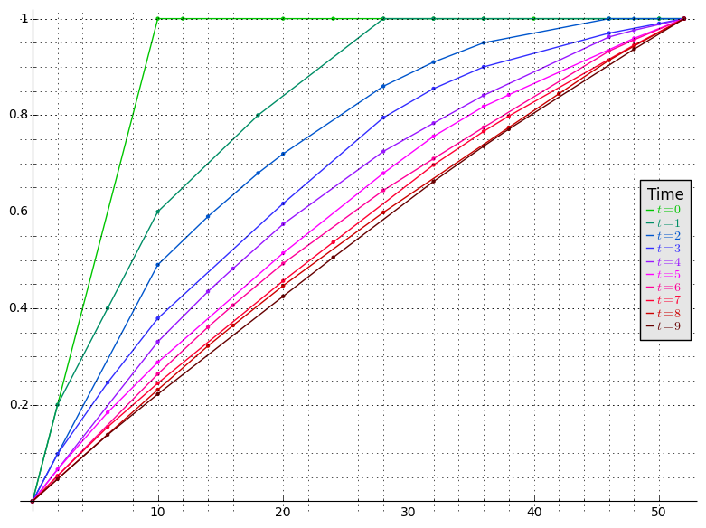
Figure 4: The function \(C^{t}\) for several values of \(t\).
We begin by showing a property of \(C^{t}\) which is closely related to concavity.
Let \(C^{t}(x)\) be the function defined above for \(x\in[4m]\) and extend it to the interval \([0,4m]\) by making it piecewise linear. Then for any \(x\) with \([x-s,x+s]\subseteq [0,4m]\) and for any \(0\leq r< s\) we have that
\begin{equation} \label{eq:rw2_Ct_property} \frac{1}{2}(C^{t}(x+s)+C^{t}(x-s))\leq\frac{1}{2}(C^{t}(x+r)+C^{t}(x-r)). \end{equation}Note that equation \eqref{eq:rw2_Ct_property} is equivalent to
\begin{equation} \nonumber C^{t}(x+s)+C^{t}(x-s)\leq C^{t}(x+r)+C^{t}(x-r). \end{equation}By the way the vertices are labeled we obtain that larger probabilities come earlier along \([0,4m]\). This implies that variation of values of \(C^{t}\) on an interval of fixed length are greater the closer the interval is to \(0\) and smaller the closer the interval is to \(4m\). Therefore, if \([x-r,x+r]\subseteq [x-s,x+s]\subseteq [0,4m]\) then
\begin{equation} \nonumber C^{t}(x+s)-C^{t}(x+r)\leq C^{t}(x-r)-C^{t}(x-s). \end{equation}Thus \(C^{t}(x+s)+C^{t}(x-s)\leq C^{t}(x+r)+C^{t}(x-r)\), as desired.
Note that taking \(r=0\) in the previous lemma implies that \(C^{t}\) is concave, that is,
\begin{equation} \nonumber C^{t}(x)\geq \frac{C^{t}(x-s)+C^{t}(x+s)}{2}, \end{equation}for all \([x-s,x+s]\subseteq[0,4m]\).
Observe that the closer \(p^{t}\) is to the stationary distribution \(\pi\), the closer the graph of \(C^{t}(x)\) is to being a line, since the probabilities are closer to being distributed equally among arcs of \(D\). Next we show the Lovász-Simonovits theorem which we will use to show that the rate of convergence of the lazy random walk is \(O(\sqrt{m})\), provided that the conductance \(\Phi(G)\) is constant.
Let \(G\) be a connected graph with conductance at least \(\phi\). Then for any probability distribution on \(V\), \(p_{0}\in \mathbb{R}^{n}\), \(t\geq 0\) and \(x\in (0,4m)\) we have that
\begin{equation} \nonumber C^{t}(x)\leq \frac{1}{2}\left( C^{t-1}(x- \phi x)+C^{t-1}(x+ \phi x)\right), \end{equation}if \(x\in (0,2m]\), and
\begin{equation} \nonumber C^{t}(x)\leq \frac{1}{2}\left( C^{t-1}(x- \phi(4m - x))+C^{t-1}(x+ \phi(4m - x))\right), \end{equation}if \(x\in [2m,4m)\).
- Split into two cases, depending on whether \(x\in (0,2m]\) or \(x\in [2m,4m)\). Further restrict \(x\) to be a breakpoint, the proof for arbitrary \(x\) follows from concavity of \(C^{t-1}\).
- Since \(x\) is a breakpoint then \(C^{t}(x)=p^{t}([k])\). Then show that \begin{equation} \nonumber p^t([k])=q_{t-1}(\text{arcs with head and tail in}[k])+q_{t-1}(\text{arcs with head or tail in}[k]) \end{equation}
- Use the property of \(C^{t}\) that for any loopless set of arcs \(A\) we have \(q_{t-1}(A)\leq \frac{1}{2}C^{t-1}(2|A|)\) together with the fact that \(e([k],V-[k])\geq \phi \deg([k])\) to deduce that \begin{equation} \nonumber C^{t}(x)\leq \frac{1}{2}\left( C^{t-1}(x- \phi x)+C^{t-1}(x+ \phi x)\right). \end{equation}
We prove the result for \(x\in (0,2m]\), the result for \(x\in[2m,4m)\) follows by an analogous argument.
First we consider the case where \(x\) is a breakpoint, say \(x=x_{k}=\sum_{i\in[k]}2d_{i}\) and let \(S=[k]\subseteq V\). Therefore \(C^{t}(x)=p^{t}(S)\).
Let \(S^{l}\) be the set of loops within \(S\), that is, \(S^{l}=\{(u,u):u\in S\}\). Denote by \(S^{o}\) the set of arcs whose tail is in \(S\), that is \(S^{o}=\{(u,v):u\in S\}\). Similarly let \(S^{i}\) denote the set of arcs whose head is in \(S\), namely \(S^{i}=\{(u,v):v\in S\}\). Observe that \(S^{o}\cap S^{i}\) is the set of arcs whose head and tail are in \(S\).
We can arrive to \(S\) from time \(t-1\) either by remaining within \(S\) via an arc of \(S^{l}\) , or by incoming to \(S\) through an arc in \(S^{i}\). Therefore
\begin{equation} \nonumber p^{t}(S)=q_{t-1}(S^{l})+q_{t-1}(S^{i}). \end{equation}Since at a given vertex there is a one to one correspondence between outgoing arcs and loops, we have that \(q_{t-1}(S^{l})=q_{t-1}(S^{o})\). Therefore
\begin{equation} \label{eq:qCrelation} \begin{split} p^{t}(S) &= q_{t-1}(S^{o})+q_{t-1}(S^{i})\\ &=q_{t-1}(S^{o}\cap S^{i})+q_{t-1}(S^{o}\cup S^{i}). \end{split} \end{equation}Now, observe that the set of arcs \(S^{o}\cap S^{i}\) contains no loops. Therefore we have
\begin{equation} \nonumber q_{t-1}(S^{o}\cap S_{i})\leq \frac{1}{2}C^{t-1}(2|S^{o}\cap S^{i}|), \end{equation}since for each arc accounted for in \(q_{t-1}(S^{o}\cap S^{i})\) there is an arc and a loop with at least its probability being accounted for in \(C^{t-1}(2|S^{o}\cap S^{i}|)\). Similarly,
\begin{equation} \nonumber q_{t-1}(S^{o}\cup S_{i})\leq \frac{1}{2}C^{t-1}(2|S^{o}\cup S^{i}|). \end{equation}Therefore from \eqref{eq:qCrelation} we derive the following inequality
\begin{equation} \nonumber p^{t}(S) \leq \frac{1}{2}(C^{t-1}(2|S^{o}\cap S^{i}|)+C^{t-1}(2|S^{o}\cup S^{i}|)). \end{equation}By noting that \(|S^{o}\cap S^{i}|=\deg(S)-e(S,V-S)\) and \(|S^{o}\cup S^{i}|=\deg(S)+e(S,V-S)\) we arrive to
\begin{equation} \nonumber p^{t}(S) \leq \frac{1}{2}\left(C^{t-1}(2(\deg(S)-e(S,V-S)))+C^{t-1}(2(\deg(S)+e(V,V-S)))\right). \end{equation}Since we assumed \(x\leq 2m\) we have that \(e(S,V-S)\geq \phi \deg(S)\) and, by the previous lemma, we conclude that
\begin{equation} \nonumber p^{t}(S)\leq \frac{1}{2}\left(C^{t-1}(2(\deg(S)-\phi\deg(S)))+C^{t-1}(2(\deg(S)+\phi\deg(S)))\right). \end{equation}Finally, since \(x_{k}=2\deg(S)\) we have that
\begin{equation} \nonumber p^{t}(S)\leq \frac{1}{2}\left(C^{t-1}(x-\phi x)+C^{t-1}(x+\phi x )\right), \end{equation}as desired. The result for \(x\in (0,2m]\) now follows from concavity of \(C^{t-1}\).
We now use the previous theorem to derive the convergence rate of the lazy random walk in terms of the conductance.
Let \(G\) be a connected graph. Then \(p^{t}(S)-\pi(S)\leq \sqrt{\deg(S)}(1-\phi^{2}/8)^{t}\)
We proceed by showing by induction on \(t\) that
\begin{equation} C^{t}(x)\leq \frac{x}{4m} + \min\{\sqrt{x}, \sqrt{4m-x}\} (1-\phi^{2}/8)^{t}, \quad\text{for all }x\in[0,4m].\label{eq:LSbound} \end{equation}Let us denote by \(U^{t}(x)\) the right hand side of the previous inequality. We prove the aove inequality for \(x\in[0,2m]\), since the argument for \(x\in[2m,4m]\) follows from an analogous argument.
First let us consider the case where \(t=0\). Observe that for \(x\in [1,2m]\) we have that \(C^{0}(x) \leq 1 \leq U^{0}(x)\). Finally for \(x\in [0,1]\) we have that \(C^{0}(x)\leq \sqrt{x}\leq U^{0}(x)\).
Now, let us assume that \eqref{eq:LSbound} holds for all \(t\leq k\). Let us show that \eqref{eq:LSbound} holds for \(t=k+1\). Let us begin by showing that
\begin{equation} \nonumber \frac{1}{2}(U^{t-1}(x-\phi x )+U^{t-1}(x+\phi x))\leq U^{t}(x). \end{equation}We have that
\begin{equation} \label{eq:LSboundU} \begin{split} \frac{1}{2}(U^{t-1}(x-\phi x )+U^{t-1}(x+\phi x)) &= \frac{x}{4m}+\frac{1}{2}\left( \sqrt{x-\phi x} + \sqrt{x + \phi x}\right)(1-\phi^{2}/8)^{t}\\ &= \frac{x}{4m}+\frac{\sqrt{x}}{2}\left( \sqrt{1-\phi} + \sqrt{1 + \phi} \right)(1-\phi^{2}/8)^{t}. \end{split} \end{equation}Considering the Taylor series of \(\sqrt{1+\phi}\) at \(\phi=0\) we have
\begin{equation} \nonumber \begin{split} \sqrt{1+\phi} &= 1+ \frac{1}{2}\phi - \frac{1}{8}\phi^{2} + \frac{1}{16} \phi^{3} - \frac{5}{128}\phi^{4}\\ &\leq 1+ \frac{1}{2}\phi - \frac{1}{8}\phi^{2}. \end{split} \end{equation}Similarly, for \(\sqrt{1-\phi}\) we obtain
\begin{equation} \nonumber \begin{split} \sqrt{1-\phi} &= 1- \frac{1}{2}\phi - \frac{1}{8}\phi^{2} - \frac{1}{16} \phi^{3} - \frac{5}{128}\phi^{4}\\ &\leq 1- \frac{1}{2}\phi - \frac{1}{8}\phi^{2}. \end{split} \end{equation}Considering the previous two inequalities we obtain the following upper bound for \eqref{eq:LSboundU}.
\begin{equation} \nonumber \begin{split} \frac{1}{2}(U^{t-1}(x-\phi x )+U^{t-1}(x+\phi x)) &\leq \frac{x}{4m} +\sqrt{x} ( 1 - \phi^{2}/8 )(1-\phi^{2}/8)^{t}.\\ &= U^{t}(x). \end{split} \end{equation}Thus, the above inequality together with the previous theorem imply that \(C^{t}(x)\leq U^{t}(x)\), as desired.
To derive the result we note that if \(S\subseteq V\) we have that
\begin{equation} \nonumber \begin{split} p^{t}(S)-\pi(S) &\leq C^{t}\left( |S| \right) - \frac{\sum_{i\in S}d_{i}}{2m} \\ &\leq \frac{\sum_{i\in S}d_{i}}{2m} + \sqrt{\sum_{i\in S}d_{i}}(1-\phi^{2}/8)^{t} - \frac{\sum_{i\in S}d_{i}}{2m}\\ &= \sqrt{\deg(S)}(1-\phi^{2}/8)^{t} \end{split} \end{equation}5.4 The Lovasz Simonovits theorem
The Lovasz Simonovits theorem is a result that is interesting by itself. In this section we provide an alternate proof of it.
We use the following notation in this section.
- \(G=(V,E)\) denotes a connected graph.
- \(W\) is the walk matrix of the lazy random walk, explicitly,
\begin{equation}
\nonumber
W=\frac{1}{2}(I+AD^{-1}).
\end{equation}
Note that \(W_{i,i}=1/2\) and that the column sum is \(1\).
It should be noted that the Lovasz Simonovits theorem is more
- \(p^{0}\in \mathbb{R}^{V}\) is a probability distribution on \(V\). The
vector \(p^{t}\) denotes the probability distribution after \(t\) steps
of the lazy random walk, recall that
\begin{equation}
\nonumber
p^{t}=Wp^{t-1}
\end{equation}
for \(t\geq 1\).
- We denote the stationary probability distribution by
\(\pi=(\pi_{1},\ldots,\pi_{n})\). Recall that this probability
distribution satisfies \(W\pi=\pi\).
- Observe that since \(W\pi=\pi\), we have that \(\sum_{j\in V}w_{i,j}\pi_{j}=\pi_{i}\). Also, since the sum of the entries of a column of \(W\) is \(1\), then \(\sum_{j\in V} w_{j,i} \pi_{i} = \pi_{i}\). Therefore \(\sum_{j\in V}w_{i,j}\pi_{j} = \sum_{j\in V} w_{j,i} \pi_{i}\).
- \(\gamma\in \mathbb{R}^{n}\) denotes the sum of the first \(k\) rows of \(W\), namely, \(\gamma = (\underbrace{1,\ldots,1}_{k\text{ ones}},0,\ldots,0)W\). Note that \(\gamma_{i}\geq 1/2\) for \(i\leq k\), and \(\gamma_{i}\leq 1/2\) for \(i\geq k\) by the structure of \(W\).
- \(F=W\Pi\), where \(\Pi=\text{diag}(\pi_{1},\ldots,\pi_{n})\). Note that
\(F\) is symmetric, since for \(ij\in E\) we have
\begin{equation}
\nonumber
f_{i,j}=W_{i,j}\pi_{j}=\frac{1}{2d_{j}}\frac{d_{j}}{2m}=\frac{1}{4m}
\end{equation}
and
\begin{equation} \nonumber f_{j,i}=W_{j,i}\pi_{i}=\frac{1}{2d_{i}}\frac{d_{i}}{2m}=\frac{1}{4m}. \end{equation}If \(ij\not\in E\) then we have \(f_{i,j}=0=f_{j,i}\).
In fact \(F\) is symmetric since \(F=W\Pi=\frac{1}{2}(I+AD^{-1})\Pi=\frac{1}{2}(\Pi + A D^{-1}\Pi) = \frac{1}{2}(\Pi + \frac{1}{2m}A)\).
By the symmetry of \(F\) it follows that for any \(S\subseteq V\) we have
\begin{equation} \nonumber \sum_{j\in V-S}(\sum_{j\in S}f_{i,j})=\sum_{i\in S}(\sum_{h\in V-S}f_{h,i}). \end{equation} - Here we define the function \(d^{t}:[0,1]\rightarrow \mathbb{R}\) which
is part of the statement of the Lovasz Simonovits theorem. We proceed
by defining two functions, \(d_{1}^{t}\) and \(d_{2}^{t}\), and showing
that they are equal, we then call this function \(d^{t}\).
Let us begin by defining \(d_{1}^{t}:[0,1]\rightarrow \mathbb{R}\). This function is defined in terms of the knapsack linear program as follows.
\begin{equation} \nonumber \begin{array}{r@{}l@{}l} d_{1}^{t}(x)= &{} \text{max} \quad &{}\sum_{i\in V}(p_{i}^{t}-\pi_{i})w_{i} \\ &{}\text{s.t.}\quad &{}\sum_{i\in V}\pi_{i}w_{i} =x \\ &{} &{} 0\leq w_{i}\leq 1, \quad i\in V. \end{array} \end{equation}Now, let us make an assumption for the definition of \(d_{2}^{t}\). Let us assume that the elements of \(V\) are labelled so that
\begin{equation} \nonumber \frac{p_{1}^{t}}{\pi_{1}} \geq \frac{p_{2}^{t}}{\pi_{2}} \geq \dots \geq \frac{p_{n}^{t}}{\pi_{n}}, \end{equation}and, assuming the ordering above, let \(\pi[k] = \sum_{i\in[k]}\pi_{i}\).
We define \(d_{1}^{t}:[0,1]\rightarrow \mathbb{R}\) as follows.
\begin{equation} \nonumber d_{2}^{t}(x)=(p_{1}-\pi_{1})+\dots+(p_{k}-\pi_{k})+\frac{x-\pi[k]}{\pi_{k+1}}(p_{k+1}-\pi_{k+1}), \end{equation}where \(k\) is such that \(\pi[k]\leq x \leq \pi[k+1]\).
We claim that \(d_{1}^{t}=d_{2}^{t}\). This follows since the optimal solution to the knapsack linear program is given by ordering the items by decreasing \(\frac{\text{profit}}{\text{size}}\) ratios and then picking as many items as to fill the knapsack.
Note that we can think of \(d^{t}\) as the function that describes how the optimal value of the knapsack linear program changes as we increase the size of the knapsack.
- Finally, let us recall the notion of conductance of a set. We define
the conductance of \(S\) as
\begin{equation}
\nonumber
\phi_{S} = \frac{ \sum_{j\in S}( \sum_{i\in V-S} w_{i,j} ) \pi_{j} }{
\min\{ \pi(S), \pi(V-S) \}} = \frac{ \sum_{j\in S}( \sum_{i\in V-S}
f_{i,j} ) }{\min\{ \pi(S), \pi(V-S) \}}.
\end{equation}
The conductance of a graph \(G\) being defined as \(\Phi=\min_{S\subseteq V}\phi_{S}\).
We are now ready to state the Lovasz Simonovits theorem.
Let \(G=(V,E)\) be a connected graph and let \(p^{0}\) be a probability distribution on \(V\). If \(d^{t}\) is defined as above then we have the following. If \(x\in[0,1/2]\) then
\begin{equation} d^{t}(x)\leq \frac{1}{2}(d^{t-1}(x-2\Phi x)+d^{t-1}(x+2\Phi x)). \label{eq:LS1} \end{equation}If \(x\in[1/2,1]\) then
\begin{equation} \nonumber d^{t}(x)\leq \frac{1}{2}(d^{t-1}(x-2\Phi (1-x))+d^{t-1}(x+2\Phi (1-x))). \end{equation}We prove the result for the case where \(x\in [0,1/2]\), the other case follows from an analogous argument. First we show that \eqref{eq:LS1} holds for the case where \(x=\pi[k]\).
If \(x=\pi[k]\) then
\begin{equation} \label{eq:gamma} \begin{split} d^{t}(x)&=\sum_{i\in k}p_{i}-\pi_{i}\\ &= (\underbrace{1,\dots,1}_{k\text{ ones}},0,\dots,0)(p^{t}-\pi)\\ &= (\underbrace{1,\dots,1}_{k\text{ ones}},0,\dots,0)(Wp^{t-1}-W\pi)\\ &= (\underbrace{1,\dots,1}_{k\text{ ones}},0,\dots,0)W(p^{t-1}-\pi)\\ &= \gamma^{\intercal}(p^{t-1}-\pi), \end{split} \end{equation}where \(\gamma\) is the sum of the first \(k\) rows of \(W\).
Let us write \(\gamma=\frac{\gamma'+\gamma''}{2}\), where \(\gamma',\gamma''\in [0,1]^{n}\). We take
\begin{equation} \gamma'_{j}= \begin{cases} 2\gamma_{j}-1 &\text{if }j\leq k\\ 0 &\text{if }j>k \end{cases},\qquad\text{ and }\qquad \gamma''_{j}= \begin{cases} 1 &\text{if }j\leq k\\ 2\gamma_{j} &\text{if }j>k \end{cases}. \end{equation}Define \(x'=(\gamma')^{\intercal}\pi\) and \(x''=(\gamma'')^{\intercal}\pi\). We then have that
\begin{equation} \label{eq:LSstep1} \begin{split} d^{t}(x)&= \gamma^{\intercal}(p^{t-1}-\pi)\\ &= \left(\frac{\gamma'+\gamma''}{2}\right)^{\intercal}(p^{t-1}-\pi)\\ &= \frac{(\gamma')^{\intercal}(p^{t-1}-\pi)+(\gamma'')^{\intercal}(p^{t-1}-\pi)}{2}. \end{split} \end{equation}Observe that \((\gamma')^{\intercal}(p^{t-1}-\pi)=x'\) so \(\gamma'\) is a feasible solution to the knapsack linear program where the knapsack has capacity \(x'\), thus \((\gamma')^{\intercal} (p^{t-1}-\pi) \leq d^{t-1}(x')\). Similarly we have \((\gamma'')^{\intercal} (p^{t-1}-\pi) \leq d^{t-1}(x'')\). Thus, from \eqref{eq:LSstep1} we get
\begin{equation} \label{eq:LSstep2} d^{t}(x)\leq \frac{d^{t-1}(x') +d^{t-1}(x'')}{2}. \end{equation}We claim that $x-x'≥ 2Φ x.$ Let us write the left hand side explicitly.
\begin{equation} \begin{split} x-x'&=\sum_{j\in V} \gamma_{j} \pi_{j} - \sum_{j\in V} \gamma_{j}' \pi_{j}\\ &=\sum_{j\leq k} (1-\gamma_{j}) \pi_{j} + \sum_{j> k} \gamma_{j} \pi_{j}\\ &=\sum_{j\leq k} \left(\sum_{i>k}w_{i,j} \right) \pi_{j} + \sum_{j> k} \left(\sum_{i\leq k}w_{i,j} \right)\pi_{j}\\ &=\sum_{j\leq k} \left(\sum_{i>k}f_{i,j} \right) + \sum_{j> k} \left(\sum_{i\leq k}f_{i,j} \right)\\ &= 2\sum_{j\leq k} \left(\sum_{i>k}f_{i,j} \right)\qquad\\ &= 2\phi_{[k]} \pi[k]. \end{split} \end{equation}And clearly the right hand side is at least \(2\Phi x\), thus the claim holds. An analogous argument shows that \(x''-x\geq 2\Phi x\).
5.5 References
This part of the notes closely follows the expositions by Lau (week 6) and Spielman (2009-lecture 8).
6 Electric networks
We use the following notation in this section
- \(G=(V,E)\) an undirected graph
- We think of each edge \(e\in E\) as a resistor with resistance \(r_{e}\). We denote the conductance of \(e\) by \(w_{e}=\frac{1}{r_{e}}\). In this same context, we call \(\sum_{v\in N(u)}w_{uv}\) the weighted degree of \(u\) and we denote it by \(d_{u}\).
- We define the weighted Laplacian \(L_{G}\) as the matrix having the \(u,v\) entry equal to \(-w_{uv}\) if \(u\neq v\) and \(d_{u}\) is \(u=v\).
- The current flowing from \(u\) to \(v\) is denoted by \(f_{u,v}\). This is a directed quantity, so \(f_{u,v}=-f_{v,u}\).
- We use \(\phi_{u}\) to denote the potential of vertex \(u\). Thus \(\phi\in\mathbb{R}^{V}\) denotes the potential of the set of vertices.
- For \(u\in V\) we define \(\chi_{u}\in \mathbb{R}^{V}\) to be the \(u\)-th standard basis vector, or the vector whose entries are all zero except entry \(u\) which is 1.
- Let \(B\) be the \(m\times n\) matrix whose rows are indexed by
edges and columns are indexed by vertices. We have that row \(uv\in
E\) of \(B\) is \(\chi_{u}-\chi_{v}\) if \(u
- Using the same indexing for the rows as above, we define the \(m\times m\) matrix \(R\) as the diagonal matrix having the conductance of the edges along the diagonal, that is, \(r_{e,e}=r_{e}\). We also let \(W=R^{-1}\).
Ohm's law (or the potential flow law) states that the potential drop across a resistor is the current flowing times the resistance, or equivalently
\begin{equation} \label{eq:ohm} f_{u,v}r_{uv}=\phi_{u}-\phi_{b} \quad\text{ or }\quad f_{u,v}=w_{uv}(\phi_{u}-\phi_{v}). \end{equation}Kirchoff's law (or the flow conservation law): The sum of the currents entering a vertex \(u\) is equal to the currents leaving \(u\), or
\begin{equation} \label{eq:kirchoff} \sum_{v\in N(u)}f_{u,v}=f_{u}, \end{equation}where \(\extCur_{u}\) denotes the external current supplied or extracted at \(u\). If current is being supplied to \(u\) then \(\extCur_{a}>0\), \(\extCur_{u}<0\) if current is being extracted from \(u\), and \(\extCur_{u}=0\) otherwise. So \(\extCur\in\mathbb{R}^{V}\).
Observe that
\begin{equation} \nonumber \begin{split} \sum_{v\in N(u)}f_{u,v} &= \sum_{v\in N(u)}w_{uv}(\phi_{u}-\phi_{v})\\ &= \sum_{v\in N(u)}w_{uv}\phi_{u}-\sum_{v\in N(u)} w_{uv}\phi_{v}\\ &= \phi_{u} d_{u} - \sum_{v\in N(u)} w_{uv}\phi_{v}. \end{split} \end{equation}Therefore \(\phi_{u} d_{u} - \sum_{v\in N(u)} w_{uv}\phi_{v} = \extCur_{u}\) for all \(u\in V\). This can be rewritten as \(L_{G}\phi = \extCur\). Therefore \(\phi = L_{G}^{-1}\extCur\). However \(L_{G}\) does not have full rank, as \(\mathbb{1}\in \ker(L_{G})\). Thus, if \(L_{G}^{+}\) denotes the pseudo-inverse of \(L_{G}\) we may compute \(\phi\) from \(\extCur\) provided \(\extCur\perp\mathbb{1}\), and in this case we have that \(\phi = L_{G}^{+}\extCur\). In general, for any \(\extCur\in \mathbb{R}^{V}\) we have that \(\phi\in\{L_{G}^{+}\extCur + \alpha\mathbb{1}:\alpha\in\mathbb{R}\}\).
Now, given the vector of potentials, we may compute the currents at each edge and the external currents at each vertex. For the currents at the edges we do this in terms of the matrices \(B\) and \(W\) defined above. We have that \(f=WB\phi\). Now, for the external currents we obtain that \(B^{t}f=\extCur\).
6.1 Effective resistance
The effective resistance between \(u\) and \(v\), \(\effResist_{u,v}\), is defined to be \(\phi_{u}-\phi_{v}\), where \(\phi\in\mathbb{R}^{V}\) is the resulting vector of potentials when one unit of current is supplied to \(u\) and one unit of current is removed from \(v\), that is, \(\extCur_{u}=1\) and \(\extCur_{v}=-1\). Intuitively we may thing of \(\effResist_{u,v}\) as the resistance between \(u\) and \(v\) given by the rest of electrical network. Algebraically we have \(L_{G}\phi=\extCur\). Now, since in this case \(\extCur=\chi_{u}-\chi_{v}\), then \(\extCur\perp\mathbb{1}\). Therefore \(\phi=L_{G}^{+ }\extCur\). As a consequence we obtain that \(\effResist_{u,v}=(\chi_{u}-\chi_{v})^{\intercal}L_{G}^{+}(\chi_{u}-\chi_{v})\).
6.2 Energy
Joule's first law asserts that the energy dissipated per unit of time at a resistor \(ab\) is given by \(f_{a,b}^{2}r_{ab}\). We define the energy dissipated in the network with currents \(f\in \mathbb{R}^E\) as the sum of all the energy dissipated at the resistors of the network, that is,
\begin{equation} \begin{split} \mathcal{E}(f)&=f^{\intercal}R f \\ &= \sum_{uv\in E}f_{u,v}^{2}r_{uv}\\ &= \sum_{uv\in E}f_{u,v}(\phi_{u}-\phi_{v})\\ &= \sum_{uv\in E}w_{ab}(\phi_{u}-\phi_{v})^{2}\\ &= \phi^{\intercal}L_{G}\phi. \end{split} \end{equation}Note that when one unit of current is supplied to \(u\) and one unit is removed from \(v\) then we have \(\effResist_{u,v}=\mathcal{E}(f)\).
Let \(g\in\mathbb{R}^{E}\) be a current assignment on \(E\) that satisfies Kirchoff's flow conservation law The next theorem, known as Thompson's Principle, shows that among all such current assignments the one minimizing the energy dissipated in the network is precisely \(f=\chi_{u}-\chi_{v}\).
For any resistor network and any two vertices \(u\) and \(v\) we have that
\begin{equation} \nonumber \effResist_{u,v}\leq \mathcal{E}(g), \end{equation}where \(g\) is defined as above.
Let \(f\) be the the flow where one unit of flow is supplied to \(u\) and one unit of flow is removed from \(v\), that is, \(f=\chi_{u}-\chi_{v}\).
Observe that \(B^{\intercal}f=\chi_{u}-\chi_{v}\) since the entry corresponding to \(x\) is given by \(\sum_{y\in N(x)}f_{x,y}=\extCur_{x}\). Similarly \(B^{\intercal}g=\chi_{u}-\chi_{v}\).
Letting \(c=g-f\) we obtain \(B^{\intercal}c=0\), this \(\sum_{y\in N(x)}c_{x,y}=0\) for all \(x\in V\). Therefore
\begin{equation} \begin{split} \mathcal{E}(g) &= \sum_{uv\in E}g_{u,v}^{2}r_{uv}\\ &= \sum_{uv\in E}(f_{u,v}+c_{u,v})^{2}r_{uv}\\ &= \sum_{uv\in E}f_{u,v}^{2}r_{uv} + 2\sum_{uv\in E}f_{u,v}c_{u,v} r_{uv}+ \sum_{uv\in E}c_{u,v}^{2}r_{uv}. \end{split} \end{equation}Note that \(\sum_{uv\in E}c_{u,v}^{2}r_{uv}\geq 0\) and by Ohm's law we have that
\begin{equation} \begin{split} \sum_{uv\in E}f_{u,v}c_{u,v} r_{uv} &= \sum_{uv\in E}(\phi_{u}-\phi_{v})c_{u,v}\\ &= \sum_{uv\in E}(\phi_{u}c_{u,v}-\phi_{v}c_{u,v})\\ &= \sum_{u\in V }\phi_{u}\sum_{uv\in E}c_{u,v}=0. \end{split} \end{equation}Therefore \(\mathcal{E}(g)\geq\mathcal{E}(f)=\effResist_{u,v}\), as desired.
6.3 Effective Resistance as Distance
It is sometimes beneficial to think of effective resistance as a measure of distance between two nodes. We can think of distance as a function \(d\) on pairs of vertices that satisfies the following properties:
- \(d(a,a) = 0\)
- \(d(a,b) \geq 0\)
- \(d(a,b) = d(b,a)\)
- \(d(a,c) \leq d(a,b) + d(b,c)\)
Our goal is to show that \(R_{eff}\) satisfies these properties, the interesting one being item 4 (the triangle inequality).
We first start with Rayleigh's monotonicity principle, which states that the effective resistance cannot decrease if we increase the resistance of some edge.
[Rayleigh's Monotonicity Principle] Let \(r\) and \(r'\) be two resistances such that \(r' \geq r\). Then \(\mathcal{E}_{r'}(f) \geq \mathcal{E}_r(f)\), where \(\mathcal{E}_r(f)\) denotes the energy of flow \(f\) under the resistances \(r\).
Let \(f\) and \(f'\) be the electric flow under resistances \(r\) and \(r'\), respectively. Then \(\mathcal{E}_{r'}(f') \geq \mathcal{E}_r(f')\) because \(r' \geq r\), and \(\mathcal{E}_r(f') \geq \mathcal{E}_r(f)\) by Thompson's principle.
We can gain some intuition about this principle by considering paths between vertices \(s\) and \(t\). If there is a short path between them, then the effetive resistance between them is ``small.'' If there are many paths between them, then the effective resistance is even smaller. More precisely, we can give the bound as stated in the following claim.
If there are \(k\) edge-disjoint paths from \(s\) to \(t\), each of lengh at most \(\ell\), then \(R_{eff}(s,t) \leq \ell/k\) (assuming the graph is unweighted).
First, note that the effective resistance between the two endpoints of \(P_n\) is \(n-1\), that is, the length of the path. It is easy to see that the graph consisting strictly of \(k\) edge-disjoint paths of length \(\ell\) between \(s\) and \(t\) has \(R_{eff}(s,t) = \ell/k\). Now, for any graph such that there are \(k\) edge-disjoint paths from \(s\) to \(t\), each of lenght at most \(\ell\), we first increase the resistances of all other edges to infinity. Then, the effective resistance is at most \(\ell/k\). By Rayleigh's Monotonicity Principle, the effective resistance in the original network could not be larger than that.
Now, we show that effictive resistance satisifies the triangle inequality.
\(R_{eff}(a,c) \leq R_{eff}(a,b) + R_{eff}(b,c)\).
Let \(\phi_{a,b}\), \(\phi_{a,c}\), and \(\phi_{b,c}\) denote the voltages when one unit of current is sent from \(a\) to \(b\), \(a\) to \(c\), and \(b\) to \(c\), respectively. So \(\phi_{a,b} = L_G^+(\chi_a-\chi_b)\), \(\phi_{a,c} = L_G^+(\chi_a-\chi_c)\), and \(\phi_{b,c} = L_G^+(\chi_b-\chi_c)\). Note that \(\phi_{a,b} + \phi_{b,c} = \phi_{a,c}\), and so,
\begin{equation} R_{eff}(a,c) = (\chi_a-\chi_c)^T \phi_{a,c} = (\chi_a-\chi_c)^T \phi_{a,b} + (\chi_a-\chi_c)^T \phi_{b,c}. \end{equation}Observe that \(\phi_{a,b}(a) \geq \phi_{a,b}(v) \geq \phi_{a,b}(b)\) (excercise?) for all \(v \in V\). It follows that,
\begin{equation} (\chi_a-\chi_c)^T \phi_{a,b} = \phi_{a,b}(a) - \phi_{a,b}(c) \leq \phi_{a,b}(a) - \phi_{a,b}(b) = R_{eff}(a,b). \end{equation}We obtain \((\chi_a-\chi_c)^T \phi_{a,b} \leq R_{eff}(b,c)\) in the same way, which then gives the claim.
6.4 References
This part of the notes closely follows the expositions by Lau (week 12) and Spielman (2010-lecture 12,2010-lecture 13).
7 Maximum Cut and the Last Eigenvalue
Given an undirected graph \(G=(V,E)\), the maximum cut problem is to find a cut \((S,\overline{S})\) that maximizes \(e(S,\overline{S})\). This is an NP-hard problem. It is easy to find a solution that cuts half of the edges. In this section, we study a non-trivial algorithm by Trevisan '09 with a 0.531-approximation factor based on the last eigenvalue of the graph.
7.1 Maximum Cut
The maximum cut problem can be formulated as an optimization problem with the objective function
\begin{equation} \nonumber \max_{S\subseteq{V}} \frac{e(S,\overline{S})}{|E|} \end{equation}which lies in \([0,1]\). The following are the optimal values for some simple graphs.
| Graphs | Maximum Cut |
| Bipartite Graphs | \(1\) |
| \(C_5\) | \(4/5\) |
| \(K_{2n}\) | \(n/(2n-1)\approx 1/2\) |
It is an exercise to show that the greedy algorithm always finds a cut of objective value at least \(1/2\). It examines the nodes in order \(1,2,\cdots,n\), and places node \(i\) in the left set \(L\) or the right set \(R\) such that at least half of the edges from \(i\) to \(\{1,2,\cdots, i-1\}\) are in the cut.
We compare the two algorithms based on linear programming and semidefinite programming in the following table.
| Based on | Approximation factor | Best possible |
| LP | 0.5 | For LP based hierarchies |
| SDP (GW '95) | 0.878 | Assuming Unique Games Conjecture |
7.2 Last Eigenvalue
The main idea in Trevisan's work is to relate the cut to the last eigenvalue of the sum Laplacian. Let \(d_{1},\ldots,d_{n}\) denote the degrees of the nodes \(1,\ldots,n\) and let \(D^{1/2}\) denote the diagonal matrix with \(D^{1/2}_{i,i}=1/\sqrt{d_{i}}\). Recall that the normalized adjacency matrix of a graph \(G\) is defined as
\begin{equation} \nonumber \hat{A}=D^{-1/2}AD^{-1/2} \end{equation}whose eigenvalues are
\begin{equation} \nonumber 1=\alpha_1\ge \alpha_2\ge \cdots \ge \alpha_n\ge -1. \end{equation}Let \(L^s\) denote the sum Laplacian
\begin{equation} \nonumber L^s=I+\hat{A} \end{equation}and
\begin{equation} \nonumber 2=\lambda_1\ge \lambda _2\ge \cdots \ge \lambda_n\ge 0 \end{equation}its eigenvalues. Let us define \(L_{e}^{s}\) for \(e=ij\) as the \(n\times n\) matrix having its \(i,i\) entry equal to \(1/d_{i}\), its \(j,j\) entry equal to \(1/d_{j}\), its \(i,j\) and \(j,i\) entries equal to \(1/\sqrt{d_{i}d_{j}}\), and \(0\) elsewhere. Note that \(L^s\) is positive semidefinite, as it is the sum of \(L_e^s\) over all edges \(e=ij\in E\), where
\begin{equation} \nonumber x^TL_e^{s}x = \frac{x_{i}^{2}}{d_{i}} + \frac{x_{j}^{2}}{d_{j}} + 2 \frac{x_{i}x_{j}}{\sqrt{d_{i}d_{j}}} = \left(\frac{x_i}{\sqrt{d_i}}+\frac{x_j}{\sqrt{d_j}}\right)^2. \end{equation}Consider a partition of the vertex set \(V\) into the left set \(L\), the right set \(R\) and the rest \(\overline{S}\). Define
\begin{equation} \nonumber \beta(L,R,\overline{S}):=\frac{\sum_{ij\in E} |y_i+y_j|}{\sum_{i} d_i |y_i|} \end{equation}where
\begin{equation} \nonumber y_i=\begin{cases} -1, \quad i\in L\\ 1, \quad i\in R\\ 0, \quad i\in \overline{S}. \end{cases} \end{equation}In Figure 5 we illustrate the motivation behind the definition of \(\beta\). We denote the number of edges having exactly one endpoint in \(\overline{S}\) to be \(\Cross\), the number of edges with exactly one endpoint in \(L\) and one endpoint in \(R\) is denoted by \(\Cut\), the number of edges having both endpoints in \(L\) or both endpoints in \(R\) is denoted by \(\Uncut\). Finally, we denote the number of edges with both endpoints in \(\overline{S}\) as \(\Deferred\). Observe how the value of \(|y_{i}+y_{j}|\) changes depending on where the edge \(ij\) has its endpoints. See Figure 5(b). We can now see that
\begin{equation} \nonumber \beta(L,R,\overline{S})=\frac{2\cdot\Uncut+\Cross}{2\cdot\Cut+2\cdot\Uncut+\Cross}. \end{equation}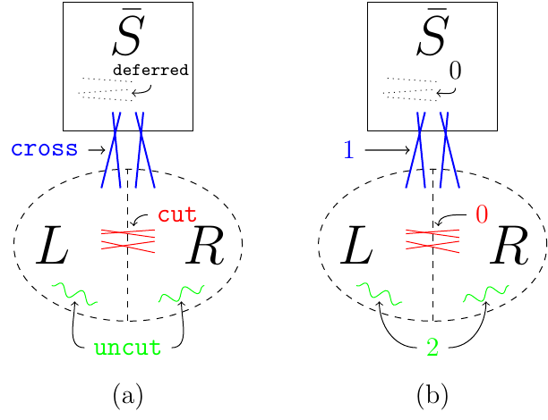
Figure 5: (a) The sets \(L\), \(R\), \(\overline{S}\), and the different types of edges given by them. (b) The value of \(|y_{i}+y_{j}|\) for each \(ij\in E\).
Let \(\beta(G)\) denote the minimum of \(\beta(L,R,\overline{S})\) over all these partitions:
\begin{equation} \beta(G):= \nonumber \min_{y\in \{-1,0,1\}^n} \frac{\sum_{ij\in E} |y_i+y_j|}{\sum_{i} d_i |y_i|}. \end{equation}Then the last eigenvalue \(\lambda_n\) provides a bound for \(\beta(G)\).
Informally speaking, \(\beta(G)\) serves as a `bridge' between \(\lambda_{n}\) and the value of \(\text{maxcut}(G)\), which is \(\max_{S\subseteq V}\frac{e(S,\overline{S})}{|E|}\). See the following proposition, which shows that if \(\text{maxcut(G)}\geq 1-\varepsilon\) then \(\beta(G)\leq \varepsilon\) and this implies \(\lambda_{n}\leq 2\varepsilon\). Before we give the proof, let us see how this set up give rise to the maximum cut algorithm.
7.3 Spectral Algorithm
The algorithm first constructs a partition \((L,R,\overline{S})\) of the vertex set \(V\) with
\begin{equation} \nonumber \beta(L,R,\overline{S})\le \sqrt{2\lambda_n} \end{equation}and then recursively solves the maximum cut problem on \(G-S\), where \(S=L\cup R\). We refer to the edges between \(L\) and \(R\) as cut edges, the ones within \(L\) or within \(R\) as uncut edges, the ones between \(S\) and \(\overline{S}\) as cross edges, and the ones within \(\overline{S}\) as deferred edges.
Maximum Cut Algorithm
Input: An undirected graph \(G=(V,E)\).
Output: An approximate maximum cut of \(G\).
- Find a 3-way partition \((L,R,\overline{S})\) of \(V\) such that \begin{equation} \nonumber \beta(L,R,\overline{S})\le \sqrt{2\lambda_n}. \end{equation}
- Iteratively find the maximum cut \((L',R')\) in deferred edges.
- Return the better cut between \((L\cup L',R\cup R')\) and \((L\cup R', R\cup L')\).
The algorithm stops when there is no cross edge or deferred edge.
7.4 Algorithm Analysis
Throughout, the partition \((L,R,\overline{S})\) satisfies
\begin{align*} \nonumber 1-\beta(L,R,\overline{S})&=1-\frac{2\cdot \Uncut + \Cross}{2\cdot \Uncut + 2\cdot\Cut+ \Cross}\\ &=\frac{\Cut}{\Uncut +\Cut+0.5\cdot \Cross}\\ &\leq \frac{\Cut +0.5\cdot \Cross}{\Uncut +\Cut+0.5\cdot \Cross + 0.5\cdot \Cross}\\ &\le \frac{\Cut}{|E-E(\overline{S})|}+\frac{0.5\cdot \Cross}{|E-E(\overline{S})|} \end{align*}By the first half of Theorem LINK MISSING, this immediately implies the following
If the maximum cut is at least \(1-\epsilon\), then \(\beta(G)\le \epsilon\), and so \(\lambda_n\le 2\epsilon\).
In other words, if \(\beta(G)>\epsilon\), then the maximum cut is of value less that \(1-\epsilon\). As a remark, \(\lambda_n\) being small does not imply that the maximum cut is large, since for any graph with a bipartite component, \(\lambda_n=0\).
By the second half of Theorem LINK TO THM MISSING,
\begin{equation} \nonumber \frac{\Cut}{|E|}+\frac{0.5\cdot \Cross}{|E|}\ge 1-\sqrt{2\lambda_n}. \end{equation}Let \(\theta\) be a parameter (later, we will fix its value to 0.1101). If \(1-\sqrt{2\lambda_n}\) is too small, say \(\lambda_n\ge \theta\), then \(\beta\ge \theta/2\), whence the optimum value is at most \(1-\theta/2\). In this case, we can choose the greedy algorithm to cut at least half edges, and this gives an approximation guarantee of
\begin{equation} \nonumber \frac{0.5}{1-0.5\cdot \theta}=\frac{1}{2-\theta} \end{equation}If \(\lambda_n<\theta\), then the spectral algorithm outputs a cut with value
\begin{equation} \nonumber \mathrm{Alg}(G)=\Cut+0.5\cdot \Cross+\mathrm{Alg}(G-S) \end{equation}Note that the optimum value satisfies
\begin{equation} \nonumber \mathrm{Opt}(G)\le \Uncut +\Cut+\Cross+\mathrm{Opt}(G-S). \end{equation}Suppose by induction that
\begin{equation} \nonumber \mathrm{Alg}(G-S)\ge \alpha\, \mathrm{Opt}(G-S). \end{equation}Then the approximation guarantee \(\gamma\) is
\begin{align*} \gamma & \ge \frac{\Cut+0.5\cdot \Cross+\alpha\,\mathrm{Opt}(G-S)}{\Uncut + \Cut+\Cross+\mathrm{Opt}(G-S)}\\ &\ge \min\left\{\frac{\Cut+0.5\cdot\Cross}{\Uncut + \Cut+\Cross},\alpha\right\}\\ &\ge \min \left\{1-\sqrt{2\theta},\alpha\right\}\\ &\ge \min\left\{1-\sqrt{2\theta},\frac{1}{2-\theta}\right\} \end{align*}If we set \(\theta=0.1107\), then the approximation guarantee is at least 0.52.
7.5 Proof of the Main Theorem
We now prove the two inequalities in Theorem LINK TO THM. We start with the easy direction.
7.5.1 Lower Bound: \(\beta(G)\ge \lambda_n/2\)
By Courant-Fischer Theorem,
\begin{equation} \nonumber \lambda_n= \min_{x\in\mathbb{R}^n} \frac{x^T L^s x}{x^Tx}= \frac{x^T\left(D^{-1/2}(D+A)D^{-1/2}\right)x}{x^Tx} \end{equation}Let \(y=D^{-1/2}x\). The above becomes
\begin{equation} \nonumber \lambda_n = \min_{y\in\mathbb{R}^n} \frac{y^T(D+A)y}{y^TDy}=\min_{y\in\mathbf{R}^n}\frac{\sum_{ij\in E} (y_i+y_j)^2}{\sum_{i}d_iy_i^2} \end{equation}Note that when \(y_i\in\{-1,0,1\}^n\), we have
\begin{gather*} (y_i+y_j)^2\le 2|y_i+y_j|\\ y_i^2=|y_i| \end{gather*}Thus
\begin{equation} \nonumber \lambda_n \le \min_{y\in\{-1,0,1\}^2} \frac{\sum_{ij\in E} 2|y_i+y_j|}{\sum_{i}d_{i}|y_i|}=2\beta(G) \end{equation}7.5.2 Upper Bound: \(\beta(G) \le \sqrt{2\lambda_n}\)
The idea of this proof is to round an eigenvector \(x\) of \(\lambda_n\) to a vector \(y\in\{-1,0,1\}^n\) randomly, so that the expected ratio
\begin{equation} \nonumber \frac{\mathbb{E}\left[\sum_{ij\in E}|y_i+y_j|\right]}{\mathbb{E}\left[\sum_{i}d_i|y_i|\right]}\le \sqrt{2\lambda_n}. \end{equation}Recall from last section that
\begin{equation} \nonumber \lambda_n=\min_{x\in\mathbb{R}^n} \frac{\sum_{ij\in E}(x_i+x_j)^2}{\sum_{i}d_ix_i^2}=\min_{x\in\mathbb{R}^n}\frac{\sum_{ij\in E}(x_i+x_j)^2}{\sum_{ij\in E}(x_i^2+x_j^2)}. \end{equation}If \(x\in\mathbb{R}^n\) is an eigenvector of \(\lambda_n\), then it attains the minimum in the above expression. When \(\lambda_n\) is sufficiently small, for an "average edge" \(ij\) such that
\begin{equation} \nonumber \frac{(x_i+x_j)^2}{x_i^2+x_j^2}=\frac{\sum_{ij\in E}(x_i+x_j)^2}{\sum_{ij\in E}(x_i^2+x_j^2)}=\lambda_n \end{equation}\(x_i\) and \(x_j\) will have different signs. Suppose \(|x_i|\ge |x_j|\). It follows that
\begin{align*} |x_i|-|x_j| &= |x_i+x_j|\\ &=\sqrt{\lambda_n(x_i^2+x_j^2)}\\ &\le \sqrt{\lambda_n}(|x_i|+|x_j|)\\ &\le 2\sqrt{\lambda_n}|x_i|. \end{align*}Thus
\begin{equation} \nonumber |x_j|\ge (1-2\sqrt{\lambda_n})|x_i|. \end{equation}Now we are ready to prove the hard direction.
By scaling the eigenvector \(x\), we may assume that \(\max_{i}x_i^2=1\). Pick \(t\in[0,1]\) uniformly at random, and round \(x\) to \(y\) with
\begin{equation} \nonumber y_i=\begin{cases} -1, \quad \text{if }x_i<0 \text{ and } x_i^2\ge t\\ 1, \quad \text{if }x_i>0 \text{ and }x_i^2\ge t\\ 0, \quad \mathrm{otherwise}. \end{cases} \end{equation}Hence \(y\) is a function of the random variable \(t\). The following argument resembles that of our proof of Cheeger's inequality from section 3.3.
- Claim: \(\mathbb{E}[|y_i|]=x_i^2\). This is because \begin{equation} \nonumber \mathbb{E}[|y_i|]=\text{Pr}[y_i^2=1]=\text{Pr}[t\le x_i^2]=x_i^2. \end{equation}
- Claim: For any edge \(ij\), we have
\begin{equation}
\nonumber
\mathbb{E}[|y_i+y_j|]\le |x_i+x_j|(|x_i|+|x_j|).
\end{equation}
To see this, we suppose \(|x_i|\ge |x_j|\) and consider two cases.
- \(x_i\) and \(x_j\) have the same sign. Then \begin{align*} \mathbb{E}[|y_i+y_j|]&=2\text{Pr}[t\le x_j^2]+\text{Pr}[x_j^2\le t\le x_i^2]\\ &=x_i^2-x_j^2+2x_j^2\\ &\leq (x_{i}+x_{j})^{2}\\ &\le|x_i+x_j|(|x_i|+|x_j|) \end{align*}
- \(x_i\) and \(x_j\) have different signs. Then \begin{align*} \mathbb{E}[|y_i+y_j|]&=\text{Pr}[x_j^2\le t\le x_i^2]\\ &=x_i^2-x_j^2\\ &=|x_i+x_j|(|x_i|+|x_j|) \end{align*}
Thus,
\begin{align} \mathbb{E}\left[\sum_{ij\in E}|y_i+y_j|\right] & \le \sum_{ij\in E}|x_i+x_j|(|x_i|+|x_j|) \nonumber\\ &\le \sqrt{\sum_{ij\in E}|x_i+x_j|^2}\sqrt{\sum_{ij\in E}(|x_i|+|x_j|)^2} \label{cauchy}\\ &= \sqrt{\lambda_n\sum_{i}d_ix_i^2}\sqrt{\sum_{ij\in E}(|x_i|+|x_j|)^2} \label{lambda}\\ &\le \sqrt{\lambda_n\sum_{i}d_ix_i^2}\sqrt{\sum_{ij\in E}2\left(x_i^2+x_j^2\right)} \nonumber\\ &=\sqrt{2\lambda_n}\left(\sum_{i}d_ix_i^2\right) \label{degree}\\ &=\sqrt{2\lambda_n}\mathbb{E}\left[\sum_{i}d_i|y_i|\right] \label{claim} \end{align}where Equation \eqref{cauchy} follows from the Cauchy–Schwarz inequality, Equation \eqref{lambda} follows from the definition of \(\lambda_n\), Equation \eqref{degree} follows from
\begin{equation} \nonumber \sum_{ij\in E}\left(x_i^2+x_j^2\right)=\sum_{i}d_ix_i^2. \end{equation}and Equation \eqref{claim} follows from the first claim. Therefore, there exists \(y\in\{-1,0,1\}^n\) such that
\begin{equation} \nonumber \frac{\mathbb{E}\left[\sum_{ij\in E}|y_i+y_j|\right]}{\mathbb{E}\left[\sum_{i}d_i|y_i|\right]}\le \sqrt{2\lambda_n} \end{equation}and so \(\beta(G)\le \sqrt{2\lambda_n}\).
7.6 References
This part of the notes closely follows the exposition by Lau (week 3).
8 Spectral Clustering
8.1 Introduction
Spectral clustering is the problem of finding clusters using spectral algorithms. Clustering is a very useful technique widely used in scientific research areas involving empirical data. As it is a natural question to ask, given a big set of data, if we can put the data into groups such that data in the same group has similar behavior. Spectral clustering often outperforms traditional clustering algorithms, as it does not make strong assumptions on the form of the clusters. In addition, it is easy to implement, and can be efficiently solved by standard linear algebra software.
In this chapter, we will focus on studying spectral clustering algorithms, and this chapter is mainly based on the survey paper by Ulrike von Luxburg (2007). We will first get familiar with the background materials related to spectral clustering, and then see two basic spectral algorithms. Afterwards, we will try to get some intuition on these spectral algorithms: why the algorithms are designed as they are. We try to rigorously justify the algorithms from graph cut point of view, perturbation theory point of view. Another theoretical justification will be given for a slightly modified spectral algorithm. Lastly, some practical details and issues will be discussed.
8.1.1 Background materials
Intuitively clustering is the problem of dividing data into groups, so that data points in the same group are more similar to each other than to those in other groups. We care about clustering problem since it gives a first impression of the data being analyzed, and is widely used in any scientific field dealing with empirical data. However, clustering is in general a hard problem. It is already NP-hard to cluster a set of vectors in a Euclidean space.
Spectral clustering is the problem of finding clusters by spectral algorithms. The basic idea is the following: First, define a graph \(G\) that captures the properties of the original data set. Then, use certain eigenvectors of a certain Laplacian of the graph \(G\) to form clusters. There are several advantages of spectral clustering: it is simple to implement and runs efficiently. Furthermore, it often outperforms traditional clustering algorithms.
Before we can run any spectral clustering algorithm on the data set, we first need to measure the "similarities" \(s_{ij}\) between each pair of data points \(x_i\), \(x_j\). We may use distance function to define the pairwise similarity: assign the similarity \(s_{ij}\) to be big if the distance between \(x_i\) and \(x_j\) is small, and assign a small similarity if their distance is big. Details will be discussed in Section Six. There are other ways to define the similarity function as well.
With the data and their pairwise similarity given, we can now define a similarity graph \(G=(V,E)\) of the data set using these information. We want this weighted graph to capture properties of the original data. It can be defined as follows: assign a vertex \(v_i\) to each data point \(x_i\), create an edge between \(v_i\) and \(v_j\) if their similarity \(s_{ij}\) is positive or bigger than a certain threshold, and take the similarity \(s_{ij}\) to be the weight of each edge \(v_iv_j\) created.
With the similarity graph, the original clustering problem is now turned into a graph partition problem. Since finding a grouping of the original data set such that different groups are dissimilar to each other in terms of similarity graph is finding a partition of the similarity graph such that the edges going between different groups have low weights.
8.2 Notations
Here are some notations that will be used later for similarity graph \(G=(V,E)\), \(V=\{v_1,\ldots , v_n\}\):
- non-negative weight of \(v_iv_j\) is defined as \(w_{ij}\).
- \(W:=(w_{ij})_{i,j=1,.,n}\) is the weighted adjacency matrix of the graph \(G\).
- \(d_i:=\sum^n_{j=1}w_{ij}\) denotes the degree of \(v_i\).
- \(D\) denotes the diagonal degree matrix of \(G\), with \(D_{ii}=d_i\) for \(i\in \{1,\ldots ,n\}\).
- \(\bar{A}\) denotes the complement of vertex set \(A\).
- \(W(A,B):= \sum_{i \in A,j \in B} w_{ij}\) is the sum of the weights of all edges going between set \(A\) and \(B\).
- \(vol(A):=\sum_{i \in A} d_i\) is a measure of the size of set \(A\).
- \(|A|\):= the cardinality of \(A\) is another measure of the size of set \(A\).
- \(\vec{1}_{A_i}\) denotes the indicator vector of set \(A_i\).
8.3 Different ways to construct the similarity graph
There are other ways to construct similarity graph of a data set in addition to the one described before:
- Fully connected graph: this similarity graph is the one described above, we create an edge between two points if their similarity \(s_{ij}\) is positive. Set \(w_{ij}=s_{ij}\) if \(v_iv_j \in E\).
- \(\epsilon\)-neighborhood graph: connect two points if their pairwise distance is smaller than \(\epsilon\). This graph is usually treated as an unweighted graph, since if \(v_iv_j \in E\), the distance between \(x_i\) and \(x_j\) is roughly of the same scale as \(\epsilon\).
- \(k\)-nearest neighbor graph: for each vertex \(v_i\), connect it to all of its \(k\)-nearest neighbors. Since this relation is not symmetric, we obtain a directed graph. The \(k\)-nearest neighbor graph is obtained by simply ignoring the directions on the edges, and set \(w_{ij}=s_{ij}\) if \(v_iv_j \in E\).
- Mutual \(k\)-nearest neighbor graph: is similar to \(k\)-nearest neighbor graph. The only difference is that after the directed graph is created, only keep edges that are bidirected, and ignore the directions. An undirected graph is obtained in this way. Set \(w_{ij}=s_{ij}\) if \(v_iv_j \in E\).
8.4 Review of graph Laplacians
Before getting into the spectral clustering algorithms, let's briefly review graph Laplacians and their basic properties:
I. Unnormalized Laplacian
The unnormalized Laplacian \(L\) is defined as \(L=D-W\). Some basic properties are as follows:
- \(f^TLf=\frac{1}{2}\sum^n_{i,j=1}w_{ij}(f_i-f_j)^2\) holds for any \(f \in \mathbb{R}^n\).
- \(L\) has \(n\) non-negative real eigenvalues: \(0=\lambda_1 \leq \lambda_2 \leq\ldots \leq \lambda_n\).
- The smallest eigenvalue of \(L\) is \(0\), and the corresponding eigenvector is \(\vec{1}\).
- The number of connected components \(A_1,\ldots ,A_k\) in graph \(G\) equals to the number of eigenvalues of \(L\) equal to \(0\), and the eigenspace of eigenvalue \(0\) is spanned by vectors \(\vec{1}_{A_1},\ldots ,\vec{1}_{A_k}\).
II. Normalized Laplacian
For our purpose, we define normalized Laplacian slightly differently here: \(L_{rw}=D^{-1}L=I-D^{-1}W\). It is denoted as \(L_{rw}\), since it is related to the random walk matrix.
It is straightforward to verify the following properties also hold for \(L_{rw}\):
- \(L_{rw}u=\lambda u\) if and only if \(\lambda\) and \(u\) solve the generalized eigenproblem \(Lu=\lambda Du\).
- \(L_{rw}\) has \(n\) non-negative real eigenvalues: \(0=\lambda_1 \leq \lambda_2 \leq\ldots \leq \lambda_n\).
- The smallest eigenvalue of \(L_{rw}\) is \(0\), and the corresponding eigenvector is \(\vec{1}\).
- The number of connected components \(A_1,\ldots ,A_k\) in graph \(G\) equals to the number of eigenvalues of \(L_{rw}\) equal to \(0\), and the eigenspace of eigenvalue \(0\) is spanned by vectors \(\vec{1}_{A_1},\ldots ,\vec{1}_{A_k}\).
8.5 Spectral clustering algorithms
Now, we are ready to see two basic spectral clustering algorithms. The first algorithm uses unnormalized Laplacian, and the second one uses normalized Laplacian. The two algorithms are very similar to each other, and the only difference is they use different graph Laplacians. However, using different graph Laplacians may lend to different outcomes of clustering. We will discuss which algorithm is more preferable at the end of Section Six.
8.5.1 Two basic spectral clustering algorithms
Before running the spectral clustering algorithms, first measure the pairwise similarities \(s_{ij}\) for each pair of data \(x_i\) and \(x_j\). Form similarity matrix \(S= (s_{ij})_{i,j=1,\ldots,n}\).
A basic unnormalized spectral clustering algorithm is as follows:
Unnormalized Spectral Clustering Algorithm Input: Similarity matrix \(S \in \R^{n\times n}\), number \(k\) of clusters to construct.
- Construct a similarity graph by one of the ways described before. Let \(W\) be its weighted adjacency matrix.
- Compute the unnormalized Laplacian \(L\).
- Compute the first \(k\) eigenvectors \(u_1,\ldots,u_k\) of \(L\).
- Let \(U \in \R^{n\times k}\) be the matrix containing the vectors \(u_1,\ldots,u_k\) as columns.
- For $i = 1,\ldots,n,$ let \(y_i \in \R^k\) be the vector corresponding to the \(i\)-th row of \(U\).
- Cluster the points \((y_i)_{i=1,\ldots ,n}\) in \(\R^k\) with \(k\)-means algorithm to obtain clusters \(C_1,\ldots,C_k\).
Output: Clusters \(A_1,\ldots ,A_k\) with \(A_i = \{j|y_j \in C_i\}\).
There are different versions of normalized spectral clustering algorithms. A basic one by Shi and Malik (2000) is as follows:
Normalized Spectral Clustering Algorithm according to Shi and Malik (2000) Input: Similarity matrix \(S \in \R^{n\times n}\), number \(k\) of clusters to construct.}
- Construct a similarity graph by one of the ways described before.} Let \(W\) be its weighted adjacency matrix.
- Compute the unnormalized Laplacian \(L\).
- Compute the first \(k\) eigenvectors \(u_1,\ldots ,u_k\) of the generalized eigenproblem \(Lu = \lambda Du\).
- Let \(U \in \R^{n\times k}\) be the matrix containing the vectors \(u_1,\ldots ,u_k\) as columns.
- For \(i = 1,\ldots ,n\), let \(y_i \in \R^k\) be the vector corresponding to the \(i\)-th row of \(U\).
- Cluster the points \((y_i)_{i=1,\ldots ,n}\) in \(\R^k\) with \(k\)-means algorithm to obtain clusters \(C_1,\ldots ,C_k\).
Output: Clusters \(A_1,\ldots ,A_k\) with \(A_i = \{j|y_j \in C_i\}\).
We see the only difference between these two algorithms is step 3. For normalized clustering algorithm, the first \(k\) eigenvectors of the generalized eigenproblem \(Lu = \lambda Du\) are exactly the first \(k\) eigenvectors of the normalized Laplacian \(L_{rw}\) if \(D\) is invertible (by the first property of normalized Laplacian). Thus, essentially the only difference between these two algorithms is they use different Laplacians to obtain the first \(k\) eigenvectors. The reason the normalized algorithm does not use \(L_{rw}\) directly is that \(L_{rw}\) is not defined when \(D\) is not invertible.
Note that the number of clusters \(k\) to be constructed is an input of the algorithms. Unfortunately, in general it is not an easy task to figure out the appropriate \(k\). A useful heuristic will be discussed in Section Six.
In both algorithms, each row of the matrix \(U\) is a vector in the Euclidean space \(\R^k\). We think of each row vector of \(U\) as a vector representation of one data point. In other words, we obtain an embedding of the original data set in \(\R^k\) by making use of the first \(k\) eigenvectors of the Laplacian. We hope this is a meaningful embedding, and when the last step of the algorithms (i.e., the \(k\)-means clustering step) is performed on this vector embedding, a clustering can be easily identified and it induces a good clustering of the original data set. We will see this is indeed the case.
8.5.2 The \(k\)-means algorithm
For completeness, we briefly introduce the \(k\)-means algorithm as in the last step of the spectral clustering algorithms.
Given a set of \(n\) vectors, \(k\)-means clustering problem aims to partition the vectors into \(k\) sets, \(S=\{S_1,\ldots S_k\}\) such that the partition minimizes the within-cluster sum of squares:
\begin{equation*} \text{min: } \sum_{i=1}^{k} \sum_{x_j \in S_i} \Norm{x_j - u_i }^2, \text{ where } u_i \text{ is the mean of vectors in } S_i. \end{equation*}\(k\)-means clustering is a NP-hard problem.
The \(k\)-means algorithm stated below is a widely used heuristic algorithm for \(k\)-means clustering. It is an iterative algorithm, and finds a clustering by the Euclidean distances between vectors. The algorithm is as follows:
\(k\)-means algorithm:
Input: \(n\) vectors, number \(k\) of clusters to be constructed.
- Randomly pick \(k\) vectors as the initial group centers.
- Assign each vector to its closest center, and obtain a grouping.
- Recalculate the centers by taking means of the groups.
- Repeat step 2 \& 3 until the centers no longer move. (i.e., the group assignment no longer changes)
In general, this algorithm runs efficiently, but there are cases the algorithm converges very slowly.
8.5.3 Illustrate by a toy example
Let's consider a toy example to get some intuition on the spectral clustering algorithms.
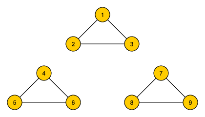
Figure 6: A toy example
Suppose a similarity graph of the original data points is constructed as in Figure 6, each edge in the graph has weight \(1\), and the input parameter \(k\) is chosen to be \(3\). Clearly, we hope the spectral clustering algorithms return three clusters: \(\{1, 2, 3\}, \{4, 5, 6\}\), and \(\{7, 8, 9\}\). Let's step through the algorithms:
Since the similarity graph has three components, by property \(4\) of both Laplacians, the first \(3\) eigenvalues are all equal to \(0\), and the first \(3\) eigenvectors are all linear combinations of \(\vec{1}_{\{1,2,3\}}, \vec{1}_{\{4,5,6\}}\) and \(\vec{1}_{\{7,8,9\}}\). As a result, all three eigenvectors are constant on \(\{1, 2, 3\}, \{4, 5, 6\}\), and \(\{7, 8, 9\}\) entries. Thus, the matrix \(U\) must have the form of:
\begin{equation*}
\left[\begin{array}{rrr}
a1&a2&a3
a1&a2&a3
a1&a2&a3
b1&b2&b3
b1&b2&b3
b1&b2&b3
c1&c2&c3
c1&c2&c3
c1&c2&c3
\end{array}\right].
\begin{equation*} As discussed before, each row of this matrix is a vector representation of a data point, so we see data points \(1,2,3\) are represented by the same vector \((a_1,a_2, a_3)\) in \(\R^3\), \(4,5,6\) are all represented by \((b_1,b_2, b_3)\), and \(7,8,9\) are all represented by \((c_1,c_2, c_3)\). Moreover, since the three eigenvectors span a \(3\)-dimensional space, \((a_1,a_2, a_3)\), \((b_1,b_2, b_3)\) and \((c_1,c_2, c_3)\) must be three distinct points in \(\R^3\). Now, if we apply the \(k\)-means clustering algorithm on this vector embedding of the data points, we will trivially get each of the three vectors as one cluster in \(\R^3\). This clustering in \(\R^3\) induces the clustering of \(\{1, 2, 3\}, \{4, 5, 6\}\), and \(\{7, 8, 9\}\) of the original data set, which is exactly the correct clustering.
By this toy example, we see the spectral algorithms do seem to capture certain fundamental properties of clustering.
8.5.4 Intuitive justification for spectral algorithms
The toy example above provides some intuitive idea why the spectral algorithms make sense. In this section, some additional intuitive justification is given.
Compare the following two facts:
- A graph \(G\) is disconnected if and only if there exist at least \(2\) eigenvalues of the Laplacians equal to \(0\). (Fact 1) This fact follows directly from the last property of both Laplacians.
- a graph \(G\) has a sparse cut if and only if there exist at least \(2\) eigenvalues of the Laplacians close to \(0\). (Fact 2) This fact follows from Cheeger's inequality. Cheeger's inequality shows that the graph conductance can be approximated by the second eigenvalue of the Laplacian. In other words, a graph has a small conductance if and only if the second eigenvalue of the graph Laplacian is small. Thus, Fact 2 follows.
It is obvious that Fact 2 is an approximate version of Fact 1.
Naturally, we may ask if there is an analogous characterization for an arbitrary \(k\). It turns out this is indeed the case. In the paper by Lee, Oveis Gharan and Trevisan (2012), it is shown that a graph \(G\) can be partitioned into \(k\) sparse cuts if and only if there exist \(k\) eigenvalues close to 0.
This shows the small eigenvalues and their eigenvectors have some strong connection with the sparse partitioning of a graph. Hence, it does make sense to use the first \(k\) eigenvectors to find clustering of the data set.
8.6 Graph cut point of view
The previous section gives some intuitive justification for the spectral algorithms. Now, let's see some rigorous justification. The first rigorous justification is from graph cut point of view.
As discussed before, with the similarity graph constructed, we turned the clustering problem into a graph partition problem. Instead of finding a clustering so that data points in the same cluster are similar to each other and points in different clusters are dissimilar to each other, we want to find a partition of the graph so that edges within a group have big weights, and edges between different groups have small weights. We will see spectral clustering algorithms are approximation algorithms to graph partition problems.
Let's first define the graph partition problem mathematically. Since the goal is to find a partition \(A_1,\ldots ,A_k\) of the graph so that there are very few edges going between different groups, we can choose the objective function to be total weights of all cut edges: cut(\(A_1,\ldots ,A_k\)):= \(\frac{1}{2}\sum_{i=1}^kW(A_i,\bar{A_i})\). The scalar of \(\frac{1}{2}\) is due to the fact every cut edge is counted twice when summing over all group cuts.
Thus, the graph partition problem is defined as: \(\underset{A_1,\ldots ,A_k}{\arg\min}\): Cut\((A_1,\ldots ,A_k)\).
Notice when \(k\) equals to \(2\), this problem is exactly the minimum cut problem. There exist efficient algorithms for this problem. However, in practice running the minimum cut algorithm in many cases only ends up separating a single vertex from the rest of the graph. This is not what we want since we want the clusters to be reasonably large sets of points.
To fix this, we require the partition to be not only sparse but balanced as well. This can be achieved by explicitly incorporating these requirements into the objective function. Instead of using total weights of cut edges as the objective function, consider RatioCut and Ncut functions as follows:
RatioCut(\(A_1,\ldots ,A_k\)):= \(\sum_{i=1}^k\frac{W(A_i,\bar{A_i})}{|A_i|}\) = \(\sum_{i=1}^k\frac{cut(A_i,\bar{A_i})}{|A_i|}\).
Ncut(\(A_1,\ldots ,A_k\)):= \(\sum_{i=1}^k\frac{W(A_i,\bar{A_i})}{vol(A_i)}\) = \(\sum_{i=1}^k\frac{cut(A_i,\bar{A_i})}{vol(A_i)}\).
The difference between the Cut function and RatioCut, Ncut functions is that in RatioCut and Ncut, each term in the sum is divided by the size of the group. The size of the group is measured by the group cardinality in RatioCut, while in Ncut, the size of the group is measured by the group volume. In this way, the requirement of having a balanced partition is incorporated into the problem as well.
Thus, we consider these two graph partition problems instead:
RatioCut graph partition problem: \(\underset{A_1,\ldots ,A_k}{\arg\min}\): RatioCut\((A_1,\ldots ,A_k)\).
Ncut graph partition problem: \(\underset{A_1,\ldots ,A_k}{\arg\min}\): Ncut\((A_1,\ldots ,A_k)\).
However, with these two objective functions the graph partition problems become NP-hard. The best we can hope for is to solve these problems approximately. Indeed, we will prove later that the unnormalized spectral clustering algorithm solves the relaxed RatioCut problem and the normalized spectral clustering algorithm solves the relaxed Ncut problem. This provides a formal justification for the spectral algorithms.
8.6.1 Approximating RatioCut
In this section, we will prove the unnormalized spectral clustering algorithm solves relaxed RatioCut problem.
The RatioCut problem is to find a partition that optimizes: \(\underset{A_1,\ldots ,A_k}{\min}\) RatioCut\((A_1,\ldots ,A_k)\). It can be rewritten in the following way:
Represent each partition \(A_1,\ldots ,A_k\) by a matrix \(H=(h_{1}|\ldots |h_{k})\in \R^{n\times k}\), where:
\begin{align*} &(h_j)_i=\begin{cases} 1/\sqrt{|A_j|} & \text{if $ v_i\in A_j$}\\ 0 & \text{otherwise} \end{cases}\hspace{0.2in} \hspace{3mm} j \in \{1,\ldots ,k\}; i \in \{1,\ldots ,n\} \hspace{7 mm} (\star) & \end{align*}By definition, it is straightforward to check that \(\{h_1,\ldots ,h_k\}\) is an orthonormal set. This implies \(H^TH=I\).
It is also easy to check the following equality:
\begin{align*}&hiTLhi=\frac{cut(Ai,\bar{A_i})}{|Ai|}\hspace{0.2in} (1)&\end{align*} {Proof of equality (1):}
\begin{align*}hiTLhi & = \frac{1}{2}∑nk,l=1wkl(hik-hil)2
& = \frac{1}{2}∑k∈ Ai,l∈ \bar{A_i}wkl(\frac{1}{\sqrt{|A_i|}}-0)2+
\frac{1}{2}∑k∈ \bar{A_i},l∈ Aiwkl(0-\frac{1}{\sqrt{|A_i|}})2
& = \frac{1}{2}\hspace{0.05in}cut(Ai,\bar{A_i}) (\frac{1}{|A_i|}) + \frac{1}{2} \hspace{0.05in} cut(Ai,\bar{A_i}) (\frac{1}{|A_i|})
& = \frac{cut(Ai,\bar{A_i})}{|Ai|}.\end{align*}
Equality (2) below is easily verifiable as well:
\begin{align*}&hiTLhi=(HTLH)ii \hspace{0.2in}\hspace{0.1in} (2)&\end{align*} With these two equalities and by definition of the trace function, we get:
RatioCut\((A_1,\ldots ,A_k) = \sum^k_{i=1}h_i^TLh_i = \sum^k_{i=1}(H^TLH)_{ii} = Tr(H^TLH)\).
Thus the problem: \(\underset{A_1,\ldots ,A_k}{\min}\) RatioCut\((A_1,\ldots ,A_k)\) can be rewritten as:
\(\underset{H\in\R^{n\times k}}{\min} Tr(H^TLH)\) s.t. \(H^TH=I, H\) as defined in (\(\star\)) for each partition.
Clearly, this is still an optimization problem over a discrete set, so it is still NP-hard. The simplest way to relax the problem is to discard the discreteness:
\(\underset{H\in\R^{n\times k}}{\min} Tr(H^TLH)\) s.t. \(H^TH=I\). This is the relaxed RatioCut problem.
Now, let's show the unnormalized spectral clustering algorithm solves this relaxed RatioCut.
By a version of the Rayleigh-Ritz theorem, we know a matrix \(U\) having the first \(k\) eigenvectors of \(L\) as its columns is an optimal solution of the relaxation. Hence, the matrix \(U\) constructed in the unnormalized spectral algorithm is an optimal solution of the relaxation.
To obtain a partition from the optimal \(U\), we consider the following two cases:
If \(U\) is one of the matrices defined as in \((\star)\) for a graph partition, then by similar arguments as in the toy example in Section Two, the unnormalized algorithm will return precisely the partition corresponding to \(U\) as the grouping when we apply the \(k\)-means step on the rows of matrix \(U\). In this case, clearly this partition is an optimal solution for the original RatioCut problem. Thus, the unnormalized algorithm solves the RatioCut problem exactly.
However, in general the optimal \(U\) is not one of the matrices defined for the graph partitions. In this case, we can still run the \(k\)-means step on the rows of \(U\) to obtain a partition. Hopefully, the partition returned is close to the optimal partition of the original RatioCut problem. Thus, the unnormalized algorithm solves the RatioCut problem approximately in this case.
Now we can conclude that the unnormalized spectral clustering algorithm solves the relaxed RatioCut problem. Note when \(k\) equals to \(2\), the spectral clustering algorithm coincides with the algorithm derived from the proof of the Cheeger's inequality.
8.6.2 Approximating Ncut
Similarly we can prove that the normalized spectral clustering algorithm solves the relaxed Ncut problem. The proof is exactly analogous to the proof of the unnormalized spectral clustering algorithm.
In this case, we represent each partition \(A_1,\ldots ,A_k\) by a matrix \(H=(h_{1}|\ldots |h_{k})\in \R^{n\times k}\), where
\begin{align*} &(h_j)_i=\begin{cases} 1/\sqrt{vol(A_j)} & \text{if $ v_i\in A_j$}\\ 0 & \text{otherwise} \end{cases}\hspace{0.2in} \hspace{3mm} j \in \{1,\ldots ,k\}; i \in \{1,\ldots ,n\}. \hspace{7 mm} & \end{align*}The rest of the proof follows in a similar fashion as in the previous section.
8.6.3 Comments on the relaxation approach
First note that there is no guarantee on the quality of the solution of the relaxed problem (i.e., the solution returned by the spectral algorithm) compared to the optimal solution of the original problem. In general, the objective difference between the two solutions can be arbitrarily large. Such example can be found in section 5.4 of von Luxburg (2007). On the other hand, we note that it is NP-hard to approximate any balanced graph partition problem with a constant approximation ratio.
There exist other relaxations for the RatioCut and Ncut problem. The relaxations shown in the previous sections are by no means unique. There are, for example, SDP relaxations as well. The advantage of the spectral relaxation is that it results in a standard linear algebra problem which is simple to solve.
8.7 Perturbation theory point of view
In this section, we rigorously justify the spectral algorithms from perturbation theory point of view. Perturbation theory is the study of how eigenvalues and eigenvectors change when a small perturbation is introduced to the matrix.
Intuitively, the justification by this approach is the following:
In the ideal situation, the similarity graph constructed represents the clustering structure of the data exactly. In this case, each connected component of the similarity graph precisely corresponds to one cluster of the original data set. With the ideal similarity graph, suppose the graph has \(k\) components, the spectral algorithms will return \(k\) clusters corresponding to the \(k\) connected components (by similar arguments as in the toy example). Clearly, in this case the spectral algorithms produce the correct clustering.
However, in real life we may not always be able to construct the ideal similarity graph. The graph constructed in real life is in general some perturbed version of the ideal graph. As a result, the Laplacians of this similarity graph are perturbed versions of the ideal Laplacians. By perturbation theory, if the perturbation is not too big and the eigengap between \(\lambda_k\) and \(\lambda_{k+1}\) of the ideal Laplacian is relatively large, then the first \(k\) eigenvectors of the perturbed Laplacian is "close to" the first \(k\) eigenvectors of the ideal one. Thus, in real life the matrix \(U\) constructed in the algorithms is "close to" the \(U\) in the ideal case. Thus, although in this case we may not have all points in a cluster being represented by the same vector, their vector representations are still relatively close to each other. Hence, after running the \(k\)-means step, the correct clustering can still be identified.
8.7.1 The rigorous perturbation argument
The above intuitive arguments can be made rigorous by Davis-Kahan theorem in perturbation theory. Let's first define some mathematical notions that are used in the theorem.
To measure the difference between two \(k\)-dimensional eigenspaces of symmetric matrices, principal angles \(\theta_i\), \(i \in \{1,\ldots ,k\}\) are generally used. They are defined as follows:
Suppose \(S_1\) and \(S_2\) are two \(k\)-dimensional subspaces of \(\R^n\) and \(V_1\) and \(V_2\) are two matrices such that their columns form orthonormal bases for \(S_1\) and \(S_2\), then the principal angles \(\theta_i\), \(i \in \{1,\ldots ,k\}\) are defined by taking the singular values of \(V_1^TV_2\) as the cosines \(cos(\theta_i)\), \(i \in \{1,\ldots ,k\}\). Note that when \(k\) equals to 1, this definition reduces to the normal angle definition between two lines in a vector space.
The matrix \(sin\Theta (S_1, S_2)\) is defined as: $\begin{pmatrix}
sin(θ1) & \hdots & 0
\vdots & \ddots & \vdots
0 & \hdots & sin(θk)
\end{pmatrix}$. We will use the Frobenius norm of this matrix to
measure the distance between subspaces \(S_1\) and \(S_2\). It is a
reasonable measure, since the bigger the angles between the
subspaces, the bigger the norm will be.
Now, we can state the Davis-Kahan theorem:
Davis-Kahan: Let \(A, H \in \R^{n \times n}\) be symmetric matrices, \(\norm {\hspace {1mm}.\hspace {1mm}}\) be the Frobenius norm of matrices, and \(\tilde A\) be \(A+H\). Let \(I_1\) be an interval in \(\R\), \(\sigma_{I_1}(A)\) be the set of eigenvalues of \(A\) in \(I_1\), and \(S_1\) be the corresponding eigenspace for these eigenvalues of \(A\). Let \(\tilde S_1\) be the analogous eigenspace for \(\tilde A\), $δ := $ min\{\(|\lambda - s|;\) \(\lambda\) eigenvalue of \(A\), \(\lambda \not \in I_1, s \in I_1\}\) be the smallest distance between \(I_1\) and the eigenvalues of \(A\) outside of \(I_1\), and let the distance between subspaces \(S_1\) and \(\tilde S_1\) be \(d(S_1, \tilde S_1):= \norm{sin\Theta (S_1, \tilde S_1)}\), then the distance \(d(S_1, \tilde S_1) \leq \frac{\norm{H}}{\delta}\).
For our purpose, we may think of the matrix \(A\) as the ideal Laplacian \(L\) (the normalized case is similar), \(H\) as a perturbation matrix, and \(\tilde A\) as the Laplacian \(\tilde L\) obtained in real life with some "noise" \(H\). Due to noise, the graph may not be completely disconnected on different clusters, but different clusters are connected by edges with low weights. In our case, we choose the interval \(I_1\) so that the first \(k\) eigenvalues of \(L\) and \(\tilde L\) are all in the interval. Thus, \(S_1\) is the eigenspace spanned by the first \(k\) eigenvectors of \(L\), and \(\tilde S_1\) is the eigenspace spanned by the first \(k\) eigenvectors of \(\tilde L\). \(\delta\) is the distance between \(I_1\) and \(\lambda_{k+1}\) of \(L\). If \(I_1\) can be chosen as \([0, \lambda_k]\), then \(\delta\) equals to the eigengap between \(\lambda_k\) and \(\lambda_{k+1}\). If the perturbation \(H\) is small, and the eigengap is large, then by Davis-Kahan theorem we have the eigenspace \(S_1\) and \(\tilde S_1\) close to each other (since their distance is bounded by \(\frac{\norm{H}}{\delta}\)).
By the same argument as before, we see the clustering the algorithm will return is close to the true clustering. By the derivation, we see the smaller the perturbation \(H\) and the bigger the spectral gap, the better the spectral algorithm works. Hence, we obtained another justification for the spectral clustering algorithms.
8.8 Justification by a slightly modified spectral algorithm
Another justification for spectral clustering is provided in this section, and it is based on the paper by Dey, Rossi and Sidiropoulos (2014). We will consider a slightly modified spectral clustering algorithm as follows:
Input: Similarity matrix \(S \in \R^{n\times n}\), number \(k\) of clusters to construct.
- Construct a similarity graph by one of the ways described before. Let \(W\) be its weighted adjacency matrix.
- Compute the normalized Laplacian \(L_{rw}\).
- Compute the first \(k\) eigenvectors \(u_1,\ldots ,u_k\) of \(L_{rw}\).
- Let \(U \in \R^{n\times k}\) be the matrix containing the vectors \(u_1,\ldots ,u_k\) as columns.
- For \(i = 1,\ldots ,n\), let \(y_i \in \R^k\) be the vector corresponding to the \(i\)-th row of \(U\). Let $f(vi) = yi $.
- Let \(R\) be a non-negative number (see Table 1 below), \(V_0 = V(G)\).
- For \(i = 1,\ldots ,k-1\), let \(v_i\) be the vertex in \(V_{i-1}\) such that the ball centered at \(f(v_i)\) with radius \(2R\) has the most number of vectors of \(f(V_{i-1})\), set \(C_i = ball(f(v_i), 2R) \cap f(V_{i-1})\), and update \(V_i = V_{i-1}\setminus C_i\) by removing previously chosen clusters.
- Set \(C_k = V_k\).
Output: Clusters \(A_1,\ldots ,A_k\) with \(A_i = \{j|y_j \in C_i\}\).
| \(R = (1-2k\sqrt{\delta})/(8k\sqrt{n})\) |
| \(\delta =1/n+ (c' \triangle ^3 k^3log^3n)/ \tau\) |
| \(\triangle =\) maximum degree of graph \(G\) |
| \(c' > 0\) is a universal constant |
| \(\tau > c'\triangle ^2 k^5log^3n\), and \(\lambda_{k+1}^3(L_{rw}) > \tau \lambda_k(L_{rw})\) |
The only difference between this spectral clustering algorithm and the ones we have seen in Section Two is that instead of using the \(k\)-means algorithm to obtain a clustering in the vector space, an approximation algorithm (by Charikar et al. 2001) for the robust \(k\)-center problem is used here.
8.8.1 Justification for this spectral clustering algorithm
The paper by Dey, Rossi and Sidiropoulos shows that for a bounded-degree graph with \(|\lambda_{k+1}-\lambda_{k}|\) (of the normalized Laplacian) large enough, this algorithm returns a partition arbitrarily close to a "strong" one. A partition of a graph is strong if each group has small external conductance and large internal conductance, which precisely characterizes a good clustering of the data set. Thus, this is another theoretical justification for spectral clustering.
The high level intuition of the paper is as follows: (for detailed theorem statements and proofs please see Dey, Rossi and Sidiropoulos, 2014)
By Oveis Gharan and Trevisan (2014), if the normalized Laplacian of a graph \(G\) has its eigengap \(|\lambda_{k+1}-\lambda_{k}|\) large enough, then there exists a graph partition into \(k\) groups, such that each group has small external conductance and large internal conductance, i.e., the partition is strong.
To prove the claim that the above algorithm returns a partition arbitrarily close to a strong one, two steps are needed. Step one involves showing that (given \(|\lambda_{k+1}-\lambda_{k}|\) is large) for each of the first \(k\) eigenvectors \(u_i\) of the Laplacian, there exists a \(\tilde u_i\) close to \(u_i\), such that \(\tilde u_i\) is constant on each group of the desired partition. Using step one, step two involves showing that (with the same assumptions) in the embedding induced by the first \(k\) eigenvectors, most groups from the desired strong partition are concentrated around center points in \(\R^k\), and different centers are sufficiently far apart from each other. Thus, when we run the approximation algorithm for the robust \(k\)-center problem, a partition arbitrarily close to a strong one is returned, so the claim follows.
8.8.2 Comments on this approach
Note this approach has similar flavor as the perturbation theory approach.
An experimental evaluation is carried out in the last section of the paper. Different graphs and different \(k\)'s are chosen to exam whether the above algorithm returns reasonable clusters. It turns out the algorithm returns meaningful clusters in all these cases, and the experiments suggest that weaker assumptions may be used in the theorems. For a complete description of the experimental result please see the paper.
Furthermore, we see from this algorithm, there is nothing principle in using the \(k\)-means algorithm as the last step for spectral algorithms. If the graph is well constructed, after the data points are embedded in the vector space, they will have well-expressed clusters so that every reasonable clustering algorithm for vectors can identify them correctly. In addition to the approximation algorithm for the robust \(k\)-center problem, there are many other techniques can be used in the last step.
8.9 Practical details and issues
Spectral clustering algorithms are very practical algorithms. In this section, we will discuss some practical details and issues related to the algorithms.
8.9.1 Construction of the similarity graph
In this section, we will discuss how to construct a good similarity graph in practice.
I. The similarity function itself
Before we can construct any similarity graph, we need to measure the pairwise similarity between each pair of data points. To obtain a meaningful similarity measure, careful choice of similarity functions is required.
In practice, the Gaussian similarity function is often used: \(s(x_i,x_j)=exp(-\norm{x_i-x_j}^2/2\sigma^2)\). This function gives a meaningful measure. Since when two data points are very close together, their similarity measure is close to \(1\), and when two points are far apart, their similarity measure is close to \(0\).
II. Which type of similarity graph
With the data set and pairwise similarity measures given, we can start constructing the similarity graph. As discussed before, there are different types of similarity graphs. It turns out the problem of choosing a suitable similarity graph for the data is a nontrivial task. Unfortunately, there is very little theoretical guidance on this matter, and the spectral algorithms are sensitive to it.
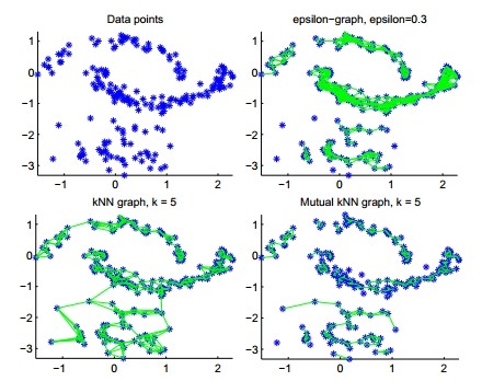
Figure 7: An example from von Luxburg (2007)
Let's illustrate the behavior of different similarity graphs by a simple example as in Figure 7 (from von Luxburg, 2007): The data set consists of vectors in \(\R^2\), with three clusters: two "moons" at top and a Gaussian at bottom shown in the upper left panel of Figure 7. The Gaussian is chosen to have a smaller density than that of the two moons.
The upper right panel shows the \(\epsilon\)-neighborhood graph constructed using \(\epsilon\) equals to \(0.3\). We see the points in the two moons are relatively well connected to the clusters they belong to. However, points in the Gaussian are barely connected to each other. As a result, when a spectral algorithm is run on this graph, the two moon clusters may be identified correctly, but the Gaussian will not be identified correctly. This is a general problem of \(\epsilon\)-neighborhood graph: it is hard to fix a parameter \(\epsilon\) which works for a data set "on different scales".
The bottom left panel shows the \(k\)-nearest neighbor graph, with \(k\) equals to \(5\). Clearly, this graph is well connected. The points are all connected to their respective clusters, and there are few edges going between different clusters. Generally, \(k\)-nearest neighbor graph can deal with data on different scales. Note the resulting Laplacians of this graph are sparse matrices, since by definition there are at most \(k\) edges adjacent to any vertex.
The bottom right panel shows the mutual \(k\)-nearest neighbor graph. We see the connectivity of this graph is somehow in between that of the previous two graphs. The Laplacian of the mutual \(k\)-nearest neighbor graph is sparse as well.
We try to avoid the use of fully connected graph, since the Laplacian of a fully connected graph is not sparse, so it will be computationally expensive.
In general, a well-connected similarity graph is preferred if it is not clear whether the disconnected components correspond to the correct clusters. Thus, the \(k\)-nearest neighbor graph is suggested as the first choice in general.
8.9.2 Computing the eigenvectors
It is seen from the last section that the Laplacian matrices of many similarity graphs are sparse. As seen in previous chapters, there exist efficient methods to compute the first \(k\) eigenvectors of a sparse matrix. For example, some popular ones include the power method and Krylov subspace methods. The speed of convergence of these methods depends on the eigengap \(|\lambda_{k+1} - \lambda_k|\) of the Laplacian. The larger the eigengap, the faster the convergence.
8.9.3 The number of clusters
As discussed before, the number \(k\) of clusters to construct is an input of the algorithms. In other words, we need to determine the number of clusters to construct before we run the algorithms. This turns out to be not an easy task.
This problem is not specifically for spectral clustering algorithms. It is a general problem for all clustering algorithms. There are many heuristics, and the eigengap heuristic is particularly designed for spectral clustering. It is the following: choose the number \(k\) such that \(\lambda_1,\ldots ,\lambda_k\) are all very small, but \(\lambda_{k+1}\) is relatively large.
Let's illustrate why this heuristic makes sense by an example (from von Luxburg, 2007) as in the figure below.
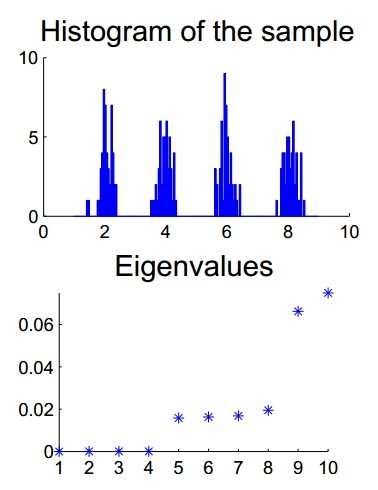
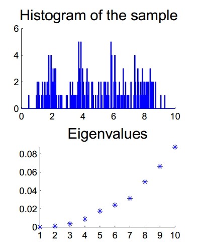
On top left, the histogram shows a data set that clearly has four clusters. We construct the \(10\)-nearest neighbor graph of the data set and compute the eigenvalues of the normalized Laplacian of the graph. The eigenvalues are plotted below the histogram. We see the first four eigenvalues are all very close to \(0\), and there is a relatively big jump from \(\lambda_4\) to \(\lambda_5\). By eigengap heuristic, this gap indicates the data set may have four clusters. The data set represented by the histogram on top right does not seem to have any clear clusters, and the plot of the eigenvalues also does not have any big eigengap, which coincides with our observation. This example shows that there is indeed some fundamental connection between the number of clusters in data set and big eigengap in the spectrum of Laplacian. Hence, this heuristic is justified.
8.9.4 Which Laplacian to use?
First note that if the similarity graph is nearly regular, using different Laplacians will not affect the outcome much. Since for a regular graph, the unnormalized Laplacian and the normalized Laplacian are only different by a multiple of identity matrix.
However, in general we encourage the use of normalized Laplacian. The reason is the following: the goal of clustering is to find clusters with small between-cluster similarity and big within-cluster similarity. In terms of similarity graph, we want a partition with small \(cut(A_i,\bar{A_i})\) and big \(vol(A_i)\) for each \(i\in\{1,\ldots ,k\}\). Observe that the Ncut graph partition problem encodes these requirements exactly since the Ncut objective is Ncut(\(A_1,\ldots ,A_k\)) = \(\sum_{i=1}^k \frac{cut(A_i,\bar{A_i})}{vol(A_i)}\). Moreover, the normalized spectral clustering algorithm solves the relaxed Ncut problem (as proved previously), so it makes sense to use normalized Laplacian to find clustering. Note that the unnormalized algorithm solves the relaxed RatioCut, but the RatioCut objective requires \(|A_i|\) instead of \(vol(A_i)\) to be small, which is not quite what we want. Hence, the use of normalized Laplacian is encouraged in general.
8.10 Conclusion
Spectral clustering algorithms have lots of applications in real life, including machine learning. However, we should apply the algorithms with care, as the algorithms are sensitive to the choice of similarity graphs, and can be unstable under different choices of parameters of the graph. Thus, the algorithms should not be taken as black boxes.
Spectral clustering is a very powerful tool, as it does not make strong assumptions on the form of the clusters. The \(k\)-means algorithm on the other hand, assumes the clusters to be of convex form, and thus may not preserve global structure of the data set. Another big advantage of spectral clustering is that it can be implemented efficiently for large data sets if the similarity graph constructed is sparse.
To further explore this subject, please refer to a list of papers in von Luxburg (2007).
9 Bipartite Ramanujan Graphs and Interlacing Families
This is a course project on the existence proof of infinite familes of bipartite Ramanujan graphs of every degree due to Marcus, Spielman and Srivastava in 2013.
9.1 Introduction
A \(d\)-regular graph is called Ramanujan if its eigenvalues are either \(\pm d\) or bounded in absolute value by \(2\sqrt{d-1}\). Ramanujan graphs have been widely used in theoretical computer science; for example, they are spectral expanders on which lazy random walks mix quickly. In (cite?), Lubotzky asked whether there exists an infinite family of Ramanujan graphs of every degree greater than two. In his earlier work with Phillips and Sarnak (cite?), and in the work by Margulis (cite?), the cases for \(d=p+1\) where \(p\) is an odd prime were solved. Later, Chiu (cite?) filled the gap for \(p=2\). Following these, Morgenstern (cite?) generalized the statement to graphs of valency \(d=q+1\) where \(q\) is a prime power. All these constructions are sproadic.
The breakthrough was made in 2013 by Marcus, Spielman and Srivastava (cite?), who proved the existence of regular Ramanujan graphs of all degrees via a probabilistic approach. They showed that the characteristic polynomials of signed adjacency matrices of a graph form an interlacing family, whence this set contains a polynomial whose roots are bounded by the largest root of the expectation over the set. By the properties of the expected characterstic polynomial, which is the well-studied matching polynomial of the graph, they bounded its largest root and thus established the existence of infinite families of regular bipartite Ramanujan graphs of all degrees. With the same method, they constructed infinite families of biregular Ramanujan graphs of all degrees. This is the first existence result on infinite families of irregular Ramanujan graphs.
In this report, we provide a detailed summary of the proof given by Marcus et al (cite?). Since most of their ideas are not restricted to regular graphs, we will stick to the general setting and work on Ramanujan graphs as defined in their paper.
9.2 General Ramanujan Graphs
Given a graph \(G\) with adjacency matrix \(A\), the spectral radius of \(G\) is
\begin{equation} \nonumber \rho(G):=\sup_{||x||_2=1} ||Ax||_2 \end{equation}where
\begin{equation} \nonumber \Vert x \Vert_2=\sum_{i=1}^{\infty}x_i^2 \end{equation}whenever the series converges. If \(G\) is finite, the spectral radius is just the largest eigenvalue of \(A\). The graph \(G\) is bipartite if and only if its smallest eigenvalue is \(-\rho(G)\). By trivial eigenvalues, we mean the eigenvalue \(\rho(G)\), and \(-\rho(G)\) when \(G\) is bipartite.
A Ramanujan graph is a graph whose non-trivial eigenvalues have small absolute values. To give an exact definition such that an infinite family of Ramanujan graphs exists, we need to know how small the non-trivial eigenvalues will stay when the graph becomes infinitely large. The answer is related to its universal cover.
The universal cover of a graph \(G=(V,E)\) is an infinite tree \(T\) with all the non-backtracking walks starting at a fixed vertex \(u\) as its vertices. Here a walk is non-backtracking if it does not contain the subsequence \(vwv\) for any \(v,w\in V\). Two vertices in \(T\) are adjacent if one is a maximal subwalk of the other, that is, if one can be obtained by appending a vertex to the other. Different graphs may have the same universal cover. For example, the universal cover of every \(d\)-regular graph is the infinite \(d\)-regular tree. We inllustrate the universal cover of the complete graph \(K_4\) on vertices \(\{1,2,3,4\}\) in Figure 8. Every vertex of \(T\) is a non-backtracking walk starting at vertex 1, denoted by the last digit in the walk sequence, as one can read off each sequence from a path starting at the root.
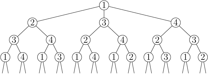 In (cite?), Greenberg proved that for every \(\varepsilon>0\) and every
infinite family of graphs that have the same universal cover \(T\),
every sufficiently large graph in the family has a non-trivial
eigenvalue that is at least \(\rho(T)-\varepsilon\). Thus, Marcus et al
(cite?) defined an arbitrary graph to be Ramanujan if its
non-trivial eigenvalues are bounded in absolute value by the
spectral radius of its universal cover. This is consistent with the
original definition of a \(d\)-regular Ramanujan graph, as the
spectral radius of an infinite \(d\)-regular tree is \(2\sqrt{d-1}\)
(cite?).
In (cite?), Greenberg proved that for every \(\varepsilon>0\) and every
infinite family of graphs that have the same universal cover \(T\),
every sufficiently large graph in the family has a non-trivial
eigenvalue that is at least \(\rho(T)-\varepsilon\). Thus, Marcus et al
(cite?) defined an arbitrary graph to be Ramanujan if its
non-trivial eigenvalues are bounded in absolute value by the
spectral radius of its universal cover. This is consistent with the
original definition of a \(d\)-regular Ramanujan graph, as the
spectral radius of an infinite \(d\)-regular tree is \(2\sqrt{d-1}\)
(cite?).
9.3 Construction
Marcus et al (cite?) realized the construction suggested by Bilu and Linial (cite?) through a sequence of 2-lifts of a base Ramanujan graph. A 2-lift of \(G=(V,E)\) is a graph with two vertices \(\{u_0,u_1\}\), called a fibre, for each vertex \(u\) in \(G\). There is a matching between two fibres \(\{u_0,u_1\}\) and \(\{v_0,v_1\}\) in the 2-lift if and only if there is an edge between \(u\) and \(v\) in \(G\). Thus, for each edge \(uv\) of \(G\), a 2-lift contains either one of the following matchings
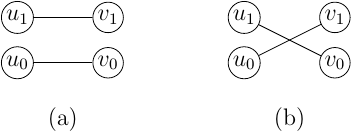
Figure 10: (a) \(\{u_0v_0,u_1v_1\}\) (b) \(\{u_0v_1,u_1v_0\}\)
Suppose there are \(m\) edges in \(G\). The signing with respect to a 2-lift is the map \(s:E\to\{1,-1\}^m\) defined by
\begin{equation} \nonumber s(uv)=\begin{cases} 1, \, \text{ if (a) appears,}\\ -1, \, \text{ if (b) appears.} \end{cases} \end{equation}If we replace the non-zero \(uv\)-entry of the adjacency matrix \(A\) by \(s(uv)\), the resulting matrix is called the signed adjacency matrix, denoted \(A_s\). In the following example, (b) is a 2-lift of the complete bipartite graph \(K_{13}\), and the corresponding signed adjacency matrix is
\begin{equation*} A_S=\begin{pmatrix}0 & \textcolor{blue}{-1} & 1 & \textcolor{blue}{-1}\\ \textcolor{blue}{-1} & 0 & 0 & 0\\ 1 & 0 & 0 & 0\\ \textcolor{blue}{-1} & 0 & 0 & 0\end{pmatrix}. \end{equation*}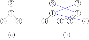
Figure 11: (a) \(K_{13}\) (b) A 2-lift of \(K_{13}\)
With the signed adjacency matrix, Bilu and Linial (cite?) characterized the eigenvalues of a 2-lift.
Let \(G\) be a graph with adjacency matrix \(A\). For a 2-lift of \(G\), let \(A_s\) be the corresponding signed adjacency matrix. The spectrum of the 2-lift is the union of the spectrum of \(A\) and the spectrum of \(A_s\).
Let \(\hat{G}\) denote the 2-lift of \(G\) and \(\hat{A}\) its adjacency matrix. Define
\begin{gather*} A_1=\frac{1}{2}(A+A_s),\\ A_{-1}=\frac{1}{2}(A-A_s). \end{gather*}Then \(\hat{A}\) can be written as
\begin{equation} \nonumber \hat{A}=\begin{pmatrix} A_1 & A_{-1}\\ A_{-1} & A_1 \end{pmatrix}. \end{equation}If \(x\) is an eigenvector of \(A\) with eigenvalue \(\lambda\), then
\begin{equation} \nonumber \hat{x}=\begin{pmatrix} x\\ x\end{pmatrix} \end{equation}is an eigenvector of \(\hat{A}\) with eigenvalue \(\lambda\). Likewise, if \(y\) is an eigenvector of \(A_s\) with eigenvalue \(\mu\), then
\begin{equation} \nonumber \hat{y}=\begin{pmatrix} y \\ -y\end{pmatrix} \end{equation}is an eigenvector of \(\hat{A}\) with eigenvalue \(\mu\). The result follows by noting that \(\hat{x}\) and \(\hat{y}\) are orthogonal.
We will refer to the eigenvalues of \(A_s\) as the new eigenvalues of the 2-lift. For a Ramanujan graph \(G\) with universal cover \(T\), if there is a 2-lift of \(G\) whose universal cover has the same spectral radius as \(T\), and whose new eigenvalues are no larger in absolute value than \(\rho(T)\), then the 2-lift is also Ramanujan. Marcus et al (cite?) showed that a weaker version of the second condition is achievable:
Every graph \(G\) with universal cover \(T\) has a 2-lift for which all of the new eigenvalues are no larger than \(\rho(T)\). \label{main}
This works as well when \(G\) is bipartite, since its eigenvalues are symemtric about zero. Further, if \(G\) is \((c,d)\)-biregular, that is, all the vertices in one colour class have degree \(c\) and all the other vertices have degree \(d\), then the first property is also satisfied, since the universal cover of every \((c,d)\)-biregular graph is the infinite \((c,d)\)-biregular tree with spectral radius \(\sqrt{c-1}+\sqrt{d-1}\) (cite?). Finally, note that a 2-lift of a bipartite graph is bipartite with the same degree distribution and thus the same universal cover. Therefore, applying 2-lifts inductively to the complete bipartite graph \(K_{cd}\), whose non-trivial eigenvlaues are zero, yields an infinite family of \((c,d)\)-biregular Ramanujan graphs.
The proof of Theorem \ref{main} is probabilistic. One attempt is to consider the expected largest eigenvalue over all signed adjacency matrices of \(G\). If the expectation were bounded by \(\rho(T)\), then so would the largest eigenvalue of some signed adjacency matrix. Unfortunately, this expectation can be much bigger than \(\rho(T)\). An alternative is to consider the expected characteristic polynomial of the signed adjacency matrices, since their roots are the new eigenvalues. In general, the relation between the roots of a sum of polynomials and the roots of a summand can be arbitrary. For reasons we will become clear with in Section \ref{interlacing}, the set of signed adjacency matrices is a spectial case, where the largest root of the expected characteristic polynomial actually provides an upper bound on the roots of some characteristic polynomial. This expectation is the matching polynomial of \(G\).
9.4 Matching Polynomials
In this section, we follow the notations of Godsil (cite?). A matching with \(r\)-edges is called an \(r\)-matching. For a graph \(G\) on \(n\) vertices, we let \(m(G,r)\) denote the number of \(r\)-matchings in \(G\). Then \(m(G,0)=1\), and \(m(G,1)\) is the number of edges in \(G\). The matching polynomial of \(G\) is the generating function
\begin{equation} \nonumber \mu(G,x)=\sum_{r\ge 0}(-1)^rm(G,r)x^{n-2r}. \end{equation}For example, the following graph has \(14\) matchings of size two and three perfect matchings, so its matching polynomial is \(x^6-8x^4+14x^2-3\).
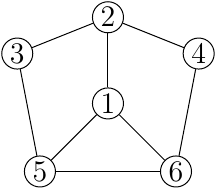
We introduce two useful properties of the matching polynomials (see, e.g, (cite?)). When we write \(G\cup H\), we mean the disjoint union of the graphs \(G\) and \(H\). The notation \(G\backslash u\) denotes the graph obtained from \(G\) with \(u\) removed, and \(G\backslash uv\) the graph obtained from \(G\) with both \(u\) and \(v\) removed.
The matching polynomial satisfies:
- \(\mu(G\cup H,x)=\mu(G,x)\mu(H,x)\),
- \(\mu(G,x)=x\mu(G\backslash u,x)-\sum_{v\sim u} \mu(G\backslash uv,x)\).
\label{prop}
- An \(r\)-matching is a disjoint union of an \(s\)-matching in \(G\) and an \(r-s\) matching in \(H\). Comparing the coefficients of \(x^{n-2r}\) in both sides yields the identity.
- If an \(r\)-matching of \(G\) does not use \(u\), then it is an
\(r\)-matching of \(G\backslash u\). If an \(r\)-matching of \(G\) uses
\(u\), then it is determined by an \((r-1)\)-matching in the
subgraph of \(G\) with \(u\) and all its neighbours removed. Thus
\begin{equation}
\nonumber
m(G,r)=m(G\backslash u,r)+\sum_{v\sim u}m(G\backslash uv,r).
\end{equation}
It follows that
\begin{align*} \mu(G,x)&=\sum_{r\ge 0}m(G,r)\\ &=x\sum_{r\ge 0}(-1)^r m(G\backslash u,r)x^{n-1-2r} \\ &\quad +(-1) \sum_{v\sim u}\sum_{r-1\ge 0} (-1)^{r-1}m(G\backslash uv,r-1)x^{n-2-2(r-1)}\\ &=x\mu(G,x)-\sum_{v\sim u}\mu(G\backslash uv,x). \end{align*}
To bound the roots of the matching polynomial of \(G\), we need a connection between the matching polynomial and the universal cover. For a vertex \(u\) in \(G\), the path tree \(P(G,u)\) is the tree with all paths in \(G\) starting at \(u\) as its vertices, such that two paths are adjacent if one is a maximal subpath of the other. Godsil proved that the matching polynomial divides the characteristic polynomial of every path tree (see, e.g, (cite?)).
Let \(P(G,u)\) be a path tree of \(G\) and \(A_P\) its adjacency matrix. The matching polynomial \(\mu(G,x)\) divides the characteristic polynomial \(\det(tI-A_P)\). In particular, all the roots of \(\mu(G,x)\) are real and bounded in absolute value by \(\rho(P(G,u))\). \label{path}
The above theorem follows from the following three lemmas and the fact that the matching polynomial and the characteristic polynomial of a forest are equal (cite?). For simplicity, we write \(\mu(G)\) for \(\mu(G,x)\) whenever the context is clear.
For a graph \(G\) and a vertex \(u\) in \(G\), let \(H\) denote the subgraph \(G\backslash u\). We have
\begin{equation} \nonumber \frac{\mu(P(H,v)\backslash v)}{\mu(P(H,v))}=\frac{\mu(P(G,u)\backslash uv)}{\mu(P(G,u)\backslash u)}. \end{equation}\label{ratio}
Let \(N\) be the set of neighbours of \(u\). If we remove \(u\) from the path tree \(P(G,u)\), the resulting graph is a forest with one component, denoted \(P_w(G,u)\backslash u\), for each vertex \(w\in N\). Thus, by the first property in Lemma \ref{prop},
\begin{equation} \mu(P(G,u)\backslash u)=\prod_{w\in N}\mu(P_w(G,u)\backslash u). \label{denom} \end{equation}Next note that the path tree \(P(H,v)\) is isomorphic to the component \(P_v(G,u)\backslash u\). Removing \(v\) from \(P(H,v)\) leaves a forest isomorphic to \(P_v(G,u)\backslash uv\). This implies
\begin{equation} \mu(P(G,u)\backslash uv)=\mu(P(H,v)\backslash v)\prod_{v\ne w\in N}\mu(P_w(G,w)\backslash u). \label{numer} \end{equation}Dividing (\ref{numer}) by (\ref{denom}) yields the result.
Let \(u\) be a vertex of \(G\) and \(P(G,u)\) be a path tree. Let \(H\) denote the subgraph \(G\backslash u\). Then
\begin{equation} \nonumber \frac{\mu(H)}{\mu(G)}=\frac{\mu(P(G,u)\backslash u)}{\mu(P(G,u))}. \end{equation}If \(G\) is a tree, then \(G=P(G,u)\). Thus we may assume inductively that the statement holds for all subgraphs of \(G\). Let \(N\) the set of neighbours of \(u\) in \(G\). By the second property in Lemma \ref{prop} and Lemma \ref{ratio},
\begin{align*} \frac{\mu(G)}{\mu(H)}&=\frac{x\mu(H)-\sum_{v\in N}\mu(H\backslash v)}{\mu(H)}\\ &=x-\sum_{v\in N}\frac{\mu(P(H\backslash v)\backslash v)}{\mu(P(H,v))}\\ &=x-\sum_{v\in N} \frac{\mu(P(G,u)\backslash uv)}{\mu(P(G,u)\backslash u)}\\ &=\frac{x\mu(P(G,u)\backslash u)-\sum_{v\in N}\mu(P(G,u)\backslash uv)}{\mu(P(G,u)\backslash u)}\\ &=\frac{\mu(P(G,u))}{\mu(P(G,u)\backslash u)}. \end{align*}Let \(P(G,u)\) be a path tree of a graph \(G\), and let \(A_P\) be the adjacency matrix of \(P(G,u)\). The matching polynomial \(\mu(G)\) divides the matching polynomial \(\mu(P(G,u))\).
Suppose that the statement holds for all subgraphs of \(G\). Since the path tree \(P(G\backslash u,v)\) is isomorphic to the component \(P_v(G,u)\backslash u\), it follows that \(\mu(P(G\backslash u,v))\) divides \(\mu(P(G,u)\backslash u)\). Now the induction hypothesis says that \(\mu(G\backslash u)\) divides \(\mu(P(G\backslash u,v))\). By Lemma \ref{ratio}, it follows that \(\mu(G)\) divides \(\mu(P(G,u))\).
Theorem \ref{path} immediately implies the following:
Let \(G\) be a graph and \(T\) its universal cover. The roots of \(\mu(G,x)\) are bounded in absolute value by \(\rho(T)\). \label{bound}
Since a path tree \(P(G,u)\) of \(G\) is a finite subgraph of \(T\), its adjacency matrix \(A_P\) is a finite submatrix of \(A_T\). By Theorem \ref{path}, the roots of \(\mu(G,x)\) are bounded in absolute value by
\begin{align*} \rho(P(G,u)) &= \sup_{||x||_2=1}||A_Px||_2\\ &= \sup_{\substack{||y||_2=1\\ \mathrm{supp}(y)\subseteq P}} ||A_Ty||_2\\ &\le \sup_{||y||_2=1} ||A_Ty||_2\\ &=\rho(T) \end{align*}Now consider the random signing \(s:E\to \{1,-1\}^m\). Let
\begin{equation} \nonumber f_s(x):=\det(xI-A_s). \end{equation}The following theorem due to Godsil and Gutman (cite?) reveals the relation between these characteristic polynomials and the matching polynomial. We present a slightly modified proof based on the one given by Marcus et al (cite?).
Let \(G\) be a graph. We have
\begin{equation} \nonumber \E(f_s(x))=\mu(G,x). \end{equation}\label{expect}
Suppose \(G\) has \(n\) vertices. For a permutation \(\sigma\in \mathrm{sym}(n)\), let \(\mathrm{sgn}(\sigma)\) denote the sign of \(\sigma\), and let
\begin{equation} \nonumber \fix(\sigma):=\{i:\sigma(i)=i\}. \end{equation}We have
\begin{equation} \nonumber \E(f_s(x))=\E\left(\sum_{\sigma\in\sym(n)}\sgn(\sigma)\prod_{i=1}^n(xI-A_s)_{i,\sigma(i)}\right). \end{equation}Expanding the above, we see that the coefficient of \(x^{n-k}\) in \(\E(f_s(x))\) is
\begin{equation} \sum_{\sigma:|\fix(\sigma)|=n-k}(-1)^k\sgn(\sigma)\E\left(\prod_{i\notin \fix(\sigma)} (A_s)_{i,\sigma(i)}\right). \label{coeff} \end{equation}Since the signings \(s(uv)\) of each edge \(uv\) are independent and \(\E(s(uv))=0\), \(\E(s(u,v)^2)=1\), the expectation
\begin{equation} \nonumber \E\left(\prod_{i\notin \fix(\sigma)} (A_s)_{i,\sigma(i)}\right)\ne 0 \end{equation}if and only if for every \(i\) not fixed by \(\sigma\), \(i\sigma(i)\) is an edge of \(G\), and \(\sigma\) decomposes into pairwise disjoint transpositions, in which case \(k\) must be even and
\begin{equation} \nonumber \{i\sigma(i):i\notin\fix(\sigma)\} \end{equation}is a perfect matching of size \(k/2\). The expectation for such \(\sigma\) reduces to
\begin{equation} \nonumber \E\left(\prod_{i\notin \fix(\sigma)} (A_s)_{i,\sigma(i)}\right)=\prod_{\substack{i\notin\fix(\sigma)\\i < \sigma(i)}}\E\left(s({i,\sigma(i)})^2\right)=1. \end{equation}It follows from (\ref{coeff}) that
\begin{equation} \nonumber \E(f_s(x))=\sum_{r\ge 0}(-1)^rm(G,r)x^{n-2r} \end{equation}which is the matching polynomial of \(G\).
Theorem \ref{bound} and Theorem \ref{expect} show that the roots of \(\E(f_s)\) are bounded by \(\rho(T)\). It suffices to prove that there is a signing \(s\) for which the largest root of \(f_s\) are bounded by the largest root of \(\E(f_s)\). This is guaranteed by the interlacing properties of \(\{f_s\}\).
9.5 Interlacing Families \label{interlacing}
Let \(g=\prod_{i=1}^{n-1}(x-\alpha_i)\) and \(f=\prod_{i=1}^n(x-\beta_i)\) be two real-rooted polynomials. We say \(g\) interlaces \(f\) if between every pair of roots of \(f\), there is a root of \(g\). In other words, \(g\) interlaces \(f\) if
\begin{equation} \nonumber \beta_1\le \alpha_1\le \beta_2\le \alpha_2\cdots\le \alpha_{n-1}\le \beta_n. \end{equation}A set of polynomials \(f_1,f_2,\cdots,f_k\) have a common interlacing if there is a polynomial \(g\) that interlaces all of them.
Let \(f_1,f_2,\cdots,f_k\) be real-rooted polynomials of the same degree that have positive leading coefficients. Let
\begin{equation*} f_{\emptyset}=\sum_{i=1}^k f_i \end{equation*}If \(f_1,f_2,\cdots,f_k\) have a common interlacing, then there exists a \(j\) such that the largest root of \(f_j\) is bounded by the largest root of \(f_{\emptyset}\). \label{common}
Suppose \(f_1,f_2,\cdots,f_k\) are of degree \(n\). Let \(\alpha_{n-1}\) be the largest root of the polynomial that interlaces all of them, and let \(\beta_n\) be the largest root of \(f_{\emptyset}\). Since all the polynomials have positive leading coefficients, \(f_i(\infty)>0\) for each \(i\). By common interlacing, it follows that \(f_i\) has exactly one root that is at least \(\alpha_{n-1}\), and thus \(f_i(\alpha_{n-1})\le 0\). As the sum, \(f_{\emptyset}(\alpha_{n-1})\le 0\), but \(f_{\emptyset}(\infty)>0\), so there is a root no smaller than \(\alpha_{n-1}\). This implies that \(\beta_n\ge \alpha_{n-1}\), and there is a \(j\) for which \(f_j(\beta_n)\ge 0\) as well. By the previous argument, there is exactly one root of \(f_j\) between \(\alpha_{n-1}\) and \(\beta_n\). Thus this must be the largest root of \(f_j\).
The characteristic polynomials \(\{f_s\}\) do not necessarily have a common interlacing. However, they still have the desired property, as we can form them into an interlacing family.
Let \(S_1,\ldots, S_m\) be \(m\) sets. Suppose we have a set of polynomials \(\{f_{s_1,\cdots, s_m}\}\) indexed by the \(m\)-tuples in \(S_1\times \cdots \times S_m\). For \(k < m\) and a partial assignment \((s_1,\cdots, s_k)\in S_1\times \cdots \times S_k\), define
\begin{equation} \nonumber f_{s_1,\cdots,s_k}:=\sum_{(s_{k+1}, \cdots, s_m)\in S_{k+1}\times \cdots \times S_m} f_{s_1,\cdots,s_k,s_{k+1},\cdots,s_m}. \end{equation}Intuitively, this is the scaled conditional expectation of the random polynomial chosen from \(\{f_{s_1,\cdots,s_m}\}\) with the first \(k\) coordinates fixed. In particular, for \(k=0\),
\begin{equation} \nonumber f_{\emptyset}:=\sum_{(s_1,\cdots, s_m)\in S_1\times \cdots \times S_m} f_{s_1,\cdots,s_m} \end{equation}which gives the expectation over the whole set.
The polynomials \(\{f_{s_1,\cdots,s_m}\}\) form an interlacing family if for every \(k < m\) and every \((s_1,\cdots,s_k)\in S_1\times \cdots \times S_k\), the polynomials
\begin{equation} \nonumber \{f_{s_1,\cdots,s_k,t}:t\in S_{k+1}\} \end{equation}have a common interlacing.
If \(\{f_{s_1,\cdots,s_m}\}\) form an interlacing family, then there exists an \(m\)-tuple \((s_1,\cdots,s_m)\) such that the largest root of \(f_{s_1,\cdots,s_m}\) is bounded by the largest root of \(f_{\emptyset}\).
We start from the set \(\{f_t:t\in S_1\}\). Since \(\{f_{s_1,\cdots,s_m}\}\) form an interlacing family, \(\{f_t:t\in S_1\}\) have a common interlacing. By Lemma \ref{common}, there is a polynomial \(f_{s_1}\) whose largest root is at most the largest root of
\begin{equation} \nonumber \sum_{t\in S_1}f_t=f_{\emptyset}. \end{equation}Having fixed the first coordinate, we consider the polynomials \(\{f_{s_1,t}: t\in S_2\}\), which also have a common interlacing. Thus there is a polynomial \(f_{s_1,s_2}\) whose largest root is at most the largest root of
\begin{equation} \nonumber \sum_{t\in S_2} f_{s_1,t}=f_{s_1}. \end{equation}Proceeding in this way, we will find the index \((s_1,\cdots,s_m)\) for which the largest root of \(f_{s_1,\cdots,s_m}\) is at most the largest root of \(f_{\emptyset}\).
A basic problem in showing a set of polynomials form an interlacing family is to prove the existence of common interlacings. This is equivalent to the problem of real-rootedness of the convex combinations of the set, as dicovered independently in (cite?).
Let \(f_1,f_2\cdots,f_k\) be polynomials of the same degree with positive leading coefficients. Then \(f_1,f_2,\cdots, f_k\) have a common interlacing if and only if \(\sum_{i=1}^k\lambda_if_i\) is real-rooted for all \(\lambda_i\ge 0\) and \(\sum_{i=1}^k\lambda_i=1\). \label{convex}
The proof of the above lemma is long. We sketch the ideas for the backward direction for two polynomials \(f\) and \(g\) with roots \(\alpha_1,\cdots,\alpha_n\) and \(\beta_1,\cdots, \beta_n\) respectively. Suppose the polynomial
\begin{equation} \nonumber h_{\lambda}=\lambda f+(1-\lambda)g. \end{equation}is real-rooted for all \(\lambda\in[0,1]\). Note that \(f_1\) and \(f_2\) have a common interlacing if and only if for each \(\ell=1,2,\cdots,n-1\), we have
\begin{equation} \nonumber \max(\alpha_{\ell},\beta_{\ell})\le \min(\alpha_{\ell+1},\beta_{\ell+1}). \end{equation}Another important observation is that that if \(f\) and \(g\) do not share any root, then the function
\begin{equation} \nonumber q_{\lambda}=\frac{\lambda}{1-\lambda}+\frac{g}{f} \end{equation}has the same roots as \(h_{\lambda}\), which are all simple. This divides the proof into three steps. First, suppose \(f\) and \(g\) have distinct roots and do not share any root. By way of contradiction, if they do not have a common interlacing, then there is a smallest \(\ell\) such that
\begin{equation} \nonumber \max(\alpha_{\ell},\beta_{\ell})> \min(\alpha_{\ell+1},\beta_{\ell+1}). \end{equation}One can show that the function \(q_0(x) < 0\) for all \(x\in(\alpha_{\ell},\alpha_{\ell+1})\). Adding a proper constant to \(q_0\) yields a funcion \(q_{\lambda}\) that has a multiple root in the interval \((\alpha_{\ell},\alpha_{\ell+1})\) for some \(\lambda\in(0,1)\). This contradicts the assumption. Next, for \(f\) and \(g\) that have multiple roots but do not share any root, the polynomials
\begin{gather*} f_{\varepsilon}=(1+\varepsilon)f+\varepsilon g\\ g_{\varepsilon}=\varepsilon f+(1-\varepsilon)g \end{gather*}with sufficiently small \(\varepsilon>0\) have simple roots as \(f\) and \(g\) respectively, and do not share any root. For any \(\lambda\in[0,1]\), the roots of
\begin{equation} \nonumber h_{\lambda,\varepsilon}=\lambda f_{\varepsilon}+(1-\lambda)g_{\varepsilon} \end{equation}are real. Thus, taking the limit for \(\varepsilon\to 0\) on both sides of
\begin{equation} \nonumber \max(\alpha_{\ell,\varepsilon},\beta_{\ell,\varepsilon})\le \min(\alpha_{\ell+1,\varepsilon},\beta_{\ell+1,\varepsilon}) \end{equation}yields
\begin{equation} \nonumber \max(\alpha_{\ell},\beta_{\ell})\le \min(\alpha_{\ell+1},\beta_{\ell+1}). \end{equation}Finally, the case where \(f\) and \(g\) with a common root \(\alpha\) can be treated by writing
\begin{gather*} f(x)=(x-\alpha)^{n_1}f_1(x)\\ g(x)=(x-\alpha)^{n_1}g_1(x) \end{gather*}and applying the second case to \(f_1\) and \(g_1\). The general statement in which \(f\) and \(g\) have more than one common root follows in a similar way.
For our characteristic polynomials \(\{f_s\}\), the sets
\begin{equation} \nonumber S_1=\cdots=S_m=\{1,-1\}. \end{equation}If for every \(k < m\) and every partial assignment \((s_1,\cdots,s_k)\in \{1,-1\}^m\), any convex combination of \(f_{s_1,\cdots,s_k,1}\) and \(f_{s_1,\cdots,s_k,-1}\) is real-rooted, then \(\{f_s\}\) form an interlacing family. This will follow from a more general result due to Marcus et al (cite?). In particular, real-rootedness of a univariate polynomial is implied by its real stability.
9.6 Real Stability
A multivariate polynomial \(f\in \mathbb{R}[z_1,\cdots,z_m]\) is called real stable if
\begin{equation} \nonumber f(z_1,\cdots,z_m)\ne 0 \end{equation}whenever the imaginary parts of all \(z_i\) are positive. Borcea and Branden (cite?) showed that the following determinantal polynomials are real stable.
Let \(A_1,\cdots,A_m\) be positive semidefinite matrices. The polynomial
\begin{equation} \nonumber \det(z_1A_1+\cdots+z_mA_m) \end{equation}is real stable. \label{det}
As a consequence of Hurwitz's theorem, if \(f(z_1,\cdots,z_m)\) is real stable, then so is \(f(z_1,\cdots,z_{m-1},c)\) for every real number \(c\) (see e.g, (cite?)). Thus, replacing any variable in the above determinantal polynomial by a real number preserves real stability.
Borcea and Branden (cite?) also characterized a class of differential operators on polynomials that preserve real stability. We will need a corollary to their characterization.
Let \(p\) and \(q\) be non-negative real numbers. Let \(u\) and \(v\) be two variables. The operator \(T=1+p\partial_u+q\partial_v\) preserves real stability. \label{T}
Operators of the above kind are of central role in the general statement that implies real-rootedness of the polynomials we are interested in. We will compose them with the operator \(Z_u\), which sets the variable \(u\) in a polynomial to zero. The following two lemmas are intermediate steps towards the general statement.
Let \(A\) be an invertible matrix, and let \(a,b\) be two vectors. Then
\begin{equation} \nonumber \det(A+ab^T)=\det(A)(1+aA^{-1}b^T). \end{equation}First,
\begin{align*} \det(A+ab^T)&=\det(A)\det(I+A^{-1}ab^T)\\ &=\det(A)\det(I+b^TA^{-1}a). \end{align*}Next note that
\begin{equation} \nonumber \begin{pmatrix} I & 0\\ b^T & 1 \end{pmatrix} \begin{pmatrix} I+ab^T & a\\ 0 & 1 \end{pmatrix} \begin{pmatrix} I & 0\\ -b & 1 \end{pmatrix} = \begin{pmatrix} I & a\\ 0 & 1+ab^T \end{pmatrix}. \end{equation}Taking the determinant of both sides yields the result.
For an invertible matrix \(A\), vectors \(a,b\), and a real number \(p\),
\begin{equation} \nonumber Z_uZ_v(1+p\partial_u+(1-p)\partial_v)\det(A+uaa^T+vbb^T)=p\det(A+aa^T)+(1-p)\det(A+bb^T) \end{equation}\label{operator}
By the matrix determinant lemma,
\begin{equation} \nonumber \partial_t\det(A+taa^T)=\det(A)(a^TA^{-1}a). \end{equation}Then
\begin{equation} \nonumber Z_uZ_vp\partial_u\det(A+uaa^T+vbb^T)=p\det(A)(a^TA^{-1}a) \end{equation}and
\begin{equation} \nonumber Z_uZ_v(1-p)\partial_v\det(A+uaa^T+vbb^T)=(1-p)\det(A)(b^TA^{-1}b). \end{equation}Now the equality follows from matrix determinant lemma.
For instance, let \(A=\begin{pmatrix}1 & 2\\ 3 & 4\end{pmatrix}\), \(a=\begin{pmatrix} 5 \\6\end{pmatrix}\) and \(b=\begin{pmatrix} 7 \\ 8\end{pmatrix}\). We have
\begin{equation} \nonumber \det(A+uaa^T+vbb^T)=4uv - 14u - 20v - 2. \end{equation}Thus
\begin{gather*} \det(A+uaa^T+vbb^T)\big|_{u=0,v=0}=-2\\ Z_uZ_v\partial_u\det(A+uaa^T+vbb^T)=4v-14\big|_{u=0,v=0}=-14\\ Z_uZ_v\partial_v\det(A+uaa^T+vbb^T)=4u-20\big|_{u=0,v=0}=-20. \end{gather*}On the other hand,
\begin{gather*} \det(A+aa^T)=-16\\ \det(A+bb^T)=-22. \end{gather*}Substituting these into both sides in Lemma \ref{operator} yields the same result \(6p-22\).
Lemma \ref{operator} leads to the main technical result on real-rootedness due to Marcus et al (cite?).
Let \(a_1,\cdots,a_m\) and \(b_1,\cdots,b_m\) be vectors in \(\mathbb{R}^n\). Let \(p_1,\cdots,p_m\) be real numbers in \([0,1]\). Let \(D\) be a positive semidefinite matrix. Then every univariate polynomial of the form
\begin{equation} \nonumber P(x):=\sum_{S\subseteq [m]} \left(\prod_{i\in S}\right) \left(\prod_{i\notin S}(1-p_i)\right)\det\left(xI+D+\sum_{i\in S} a_ia_i^T+\sum_{i\notin S} b_ib_i^T\right) \end{equation}is real-rooted. \label{technical}
Define a determinantal polynomial on variables \(x,u_1,\cdots,u_m,v_1,\cdots,v_m\):
\begin{equation} \nonumber Q(x,u_1,\cdots,u_m,v_1,\cdots,v_m)=\det\left(xI+D+\sum_i u_ia_ia_i^T+\sum_i v_ib_ib_i^T\right). \end{equation}Lemma \ref{det} shows that \(Q\) is real stable. By Lemma \ref{operator} and induction,
\begin{equation} \nonumber P(x)=\left(\prod_{i=1}^mZ_{u_i}Z_{v_i}T_i\right)Q(x,u_1,\cdots,u_m,v_1,\cdots,v_m). \end{equation}From Lemma \ref{T}, applying \(Z_{u_i}Z_{v_i}T_i\) to \(Q\) preserves stability. Thus \(P(x)\) is a univariate real stable polynomial. Since the complex roots of a real polynomial come in conjugate pairs, it follows that \(P(x)\) is real-rooted.
Now we show that if we pick the sign for each edge independently with any probability \(p_i\), then the expected characteristic polynomial is still real-rooted.
Let \(p_1,\cdots,p_m\) be numbers in \([0,1]\). Then the following polynomial is real-rooted
\begin{equation} \sum_{s\in\{\pm 1\}^m} \left(\prod_{i:s_i=1} p_i\right)\left(\prod_{i:s_i=-1}(1-p_i)\right) f_s(x). \end{equation}\label{real-rooted}
Let \(d\) be the maximum degree of the graph \(G\). It is equivalent to show that
\begin{equation} \nonumber \sum_{s\in\{\pm 1\}^m} \left(\prod_{i:s_i=1} p_i\right)\left(\prod_{i:s_i=-1}(1-p_i)\right) \det(xI+dI-A_s). \label{trans} \end{equation}is real-rooted. Let \(D\) be the diagonal matrix with \(D_{uu}=d-d(u)\), where \(d(u)\) is the degree of the vertex \(u\), and let \(L\) be the Laplacian matrix of \(G\). Then \(D\) is positive semidefinite and
\begin{equation} \nonumber dI-A_s=L+D \end{equation}Further, \(L\) can be written as
\begin{equation} \nonumber L=\sum_{uv\in E}L_{uv}^{s(uv)} \end{equation}where
\begin{gather*} L_{uv}^1=(e_u-e_v)(e_u-e_v)^T\\ L_{uv}^{-1}=(e_u+e_v)(e_u+e_v)^T. \end{gather*}Thus by Theorem \ref{technical}, the polynomial in (\ref{trans}) is real-rooted.
9.7 Main Results
In this section, we prove the interlacing property of \(\{f_s\}\), which leads to the final existence result (cite?).
The polynomials \(\{f_s\}\) form an interlacing family.
For every \(k < m\) and \(\lambda\in[0,1]\), apply Theorem \ref{real-rooted} with
\begin{equation} \nonumber p_i=\frac{1+s_i}{2}, \quad i=1,\cdots,k \end{equation}and
\begin{equation} \nonumber p_{k+1}=\lambda, p_{k+2}=\cdots=p_m=\frac{1}{2}. \end{equation}Then the convex combination
\begin{equation} \nonumber \lambda f_{s_1,\cdots,s_k,1}(x)+(1-\lambda)f_{s_1,\cdots,s_k,-1}(x) \end{equation}is real-rooted for every partial assignment \((s_1,\cdots,s_k)\in \{1,-1\}^k\). By Lemma \ref{convex}, the polynomials \(\{f_s\}\) are an interlacing family.
For every \(c,d\ge 3\), there is an infinite sequence of \((c,d)\)-biregular bipartite Ramanujan graphs.
Apply 2-lift construction inductively to the complete bipartite graph \(K_{c,d}\). By Theorem \ref{main}, every \((c,d)\)-biregular Ramanujan graph \(G\) has a 2-lift whose new eigenvalues are bounded by \(\sqrt{c-1}+\sqrt{d-1}\), the spectral radius of the universal cover of \(G\). Since the 2-lift is bipartite and \((c,d)\)-biregular, its also Ramanujan.
9.8 Future Work
Marcus et al (cite?) proved the existence of infinite families of biregular Ramanujan graphs of all degrees. In particular, this answers Lubotzy's question on the existence of infinite families of \(d\)-regular Ramanujan graph for every \(d\ge 3\) (cite?). However, the application of Theorem \ref{main} is restricted to bipartite graphs, as it only provides an upper bound on the eigenvalues. It will be interesting to find a construction of non-bipartite Ramanujan graphs.
Another challenge is to give an efficient algorithm that finds the desired family of bipartite Ramanujan graphs. The existence proof in (cite?) is probabilistic, in which the polynomials \(\{f_{s_1,\cdots,s_k,t}\}\) are not easy to compute. For example, computing the matching polynomial of a graph is a \(\sharp P\)-hard problem in general. Thus, one might want to discover a polynomial-time algorithm based on this method.
10 Improved Cheeger's Inequality
10.1 Introduction
In the course, we saw the proof of Cheeger's inequality:
For a connected graph \(G\) we have:
\begin{equation} \frac{1}{2} \lambda _2 \leq \phi(G) \leq \sqrt{2 \lambda_2}, \label{e1} \end{equation}where \(\phi(G)\) is the conductance of the graph and \(\lambda_2\) is the second smallest eigenvalue of the normalized Laplacian matrix.
The proof of the Cheeger's inequality is constructive and gives a spectral partitioning algorithm: take an eigenvector \(f\) of \(\lambda_2\), consider all the canonical cuts introduced by \(f\) and pick one with the smallest conductance. Let \(\phi(f)\) be the corresponding smallest conductance. The proof of the Cheeger's inequality actually shows that \(\frac{1}{2} \lambda _2 \leq \phi(f) \leq \sqrt{2 \lambda_2}\). Therefore, the spectral partitioning algorithm gives a linear time \(O(1/\sqrt{\lambda_2})\)-approximation algorithm for finding a sparse cut. However, the worst case performance is bad as \(\lambda_2\) can be as small as \(1/n^2\).
Spectral partitioning is a popular heuristic algorithm as it is easy to implement and works really good for some applications such as image segmentation and clustering. Its performance is much better than the worst case performance guaranteed by Cheeger's inequality and little explanation has been found for it. Improved Cheeger's inequality is a good step towards finding theoretical explanation for these kind of phenomena. It improves the upper bound of the Cheeger's inequality by using higher order spectral information. Improved Cheeger's inequality can also be used to find \(k\)-way graph partitioning that is partitioning the vertices of a graph into \(k\) disjoint sets such that the maximum conductance among them is small.
In Section 2, we see some preliminary results and definitions and also the statement of the improved Cheeger's inequality. In Section 3, we prove the main theorem. Section 4 is about spectral max cut algorithms. In class, we saw Trevisan's spectral algorithm for finding the maximum cut of a graph with approximation guarantee slightly more than \(0.5\). In the same fashion as improved Cheeger's inequality, in Section 4, we see an improved bound using higher order spectral information. Using that, we introduce another max cut algorithm that actually uses higher order spectral information. Section 5 is the conclusion.
10.2 Preliminary definitions and results
Assume that we have a connected graph \(G=(V,E,w)\), with positive weights on the edges. For two sets of vertices \(S\) and \(T\), we define \(E(S,T)\) as the set of all edges that has one end in \(S\) and the other end in \(T\), we also define \(E(S)=E(S,S)\). We can extend the definition of weight to vertices as \(w(v)=\sum_{u \sim v} w(u,v)\), for all \(v \in V\). Note that if we use unit weights, then the weight of each vertex is just the degree of that. We define the volume of any \(S \subseteq V\) as \(vol(S):= \sum_{v \in S} w(v)\). Given a subset of vertices \(S\), we define the conductance of \(S\) as
\begin{equation} \nonumber \phi(S) := \frac{w(E(S, \overline{S}))}{\min \{vol(S),vol(\overline{S})\} }. \end{equation}For a vector \(f \in \mathbb R^V\), and for a threshold \(t \in \mathbb R\), let \(V_f(t) := \{v: f(v) \geq t\}\) be a threshold set of \(f\). We let
\begin{equation} \phi(f) := \min_{t \in \mathbb R} \phi(V_f(t)). \label{phi-f} \end{equation}We define the adjacency matrix as an operator that for any vector \(f \in \mathbb R^V\) and any vertex \(v\), we have \(Af(v) = \sum_{u \sim v} w(u,v) f(u)\). We also define the diagonal matrix \(D\) with the weights of vertices \(w(v)\)'s on the diagonal. Then the normalized Laplacian matrix is
\begin{equation} \nonumber \mathcal{L}:= I - D^{-1/2} A D^{-1/2}. \end{equation}\(\mathcal{L}\) is a positive semidefinite matrix with eigenvalues:
\begin{equation} \nonumber 0 = \lambda_1 \leq \lambda_2 \leq \ldots \leq \lambda_n \leq 2. \end{equation}Here is the statement of the main theorem, improved Cheeger's inequality, we prove.
For any undirected graph \(G\) and an eigenvector \(f\) of \(\lambda_2\), we have:
\begin{equation} \phi(G) \leq \phi (f) = O(k) \frac{\lambda_2}{\sqrt{\lambda_k}}, \ \ \ k \geq 2. \end{equation}\label{T1}
The above theorem is interesting because it gives an improved theoretical bound for spectral partitioning algorithm that contains \(\lambda_k\), but the algorithm does not use any information from higher order eigenvalues. Informally, improved Cheeger's inequality shows that the graph has at most \(k-1\) outstanding sparse cuts when \(\lambda_{k-1}\) is small and \(\lambda_k\) is large. Let us see an example here. Let \(G\) be a graph on 50 vertices constructed as follows: attach a copy of a complete graph \(K_{10}\) to each vertex of a 5-cycle as in Figure \ref{Fig1}.
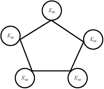
Figure 13: Graph \(G\) on 50 vertices.
The first 6 eigenvalues of the normalized Laplacian are
\begin{equation} \nonumber \lambda_1=0, \ \ \lambda_2=\lambda_3=0.0134, \ \ \lambda_4=\lambda_5=0.0297, \ \ \lambda_6=0.9293. \end{equation}As can be seen, there are 5 major components in graph \(G\). In other words, we can partition \(V(G)\) into 5 disjoint sets with small conductances. However, it is easy to check that we cannot partition it into 6 disjoint sets with the same property. Improved Cheeger's inequality implies that there is a large gap between \(\lambda_5\) and \(\lambda_6\) as can be seen above. Another interesting observation is an eigenvector of \(\lambda_2\). Figure \ref{Fig2} shows an eigenvector of \(\lambda_2\) as a functional of vertices. As can be seen, the eigenvector is like a step function. This is a key idea in the proof of the main theorem that if there is large gap between \(\lambda_{k-1}\) and \(\lambda_k\) for a small \(k\), then the second eigenvector is close to a step function, with \(O(k)\) number of steps. This also gives us an idea on \(k\)-way graph partitioning.
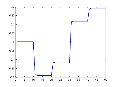
Figure 14: An eigenvector of \(\lambda_2\) as a functional of vertices.
Informally, improved Cheeger's inequality says
- An undirected graph has \(k\) disjoint sparse cuts if and only if \(\lambda_k\) is small.
- When \(\lambda_{k-1}\) is small and \(\lambda_k\) is large, we can partition the graph into \(k-1\) sets of small conductance, but for every partitioning into \(k\) sets, there exists a set with large conductance.
Let us define the weighted norm of a vector \(f\) and its Rayleigh quotient with respect to \(G\) as
\begin{equation} \|f\|^2_w:=\sum_{v\in V} w(v) f^2(v), \ \ \ \ \mathcal{R}(f):=\frac{\sum_{uv \in E} w(u,v) |f(u)-f(v)|^2}{\|f\|_w^2}. \end{equation}The support of a vector \(f\) is defined as \(\text{supp}(f) := \{v, f(v) \neq 0\}\).
In the rest of this section, we see three lemmas needed for the proof of the main theorem. The proof starts with the following lemma:
There exists a non-negative functional \(f\) with \(\|f\|_w^2=1\) such that \(\mathcal{R}(f) \leq \lambda_2\) and \(vol(supp(f)) \leq vol(V)/2\). \label{R1}
Let \(g\) be a second eigenvector for \(\mathcal{L}\). Let \(g_+\) and \(g_-\) be such that \(g_+(u)=\max\{g(u),0\}\) and \(g_-(u)=\min\{g(u),0\}\). Let us first consider \(g_+\): for any vertex \(u \in \text{supp}(g_+)\), we can write:
\begin{equation} \nonumber (\mathcal{L}g_+)(u) = g_+(u) - \sum_{v:v \sim u} \frac{w(u,v) g_+(u)}{\sqrt{w(u)w(v)}} \leq g(u) - \sum_{v:v \sim u} \frac{w(u,v) g(u)}{\sqrt{w(u)w(v)}} = (\mathcal{L}g)(u)=\lambda_2 g(u). \end{equation}The first inequality is from the fact that \(g_+(u)=g(u)\) as \(u \in \text{supp}(g_+)\) and the fact that the positive entries of \(g\) and \(g_+\) are the same, but \(g\) might have some negative entries as well. Using the above inequality, we have
\begin{equation} \nonumber \langle g_+,\mathcal{L}g_+ \rangle = \sum_{u \in \text{supp}(g_+)} g_+(u)( \mathcal{L}g_+)(u) \leq \sum_{u \in \text{supp}(g_+)} \lambda_2 g_+(u)^2 = \lambda_2 \|g_+\|^2. \end{equation}By defining \(f_+=D^{-1/2}g_+\), we get
\begin{equation} \nonumber \lambda_2 \geq \frac{\langle g_+, \mathcal{L}g_+ \rangle}{\|g_+\|^2} = \frac{\langle f_+,(D-A)f_+ \rangle}{\|f_+\|_w^2}=\mathcal{R}(f_+). \end{equation}Similarly, we can define \(f_-=D^{-1/2}g_-\), and show that $\mathcal{R}(f_-)≤ λ2 $. Now at least one of \(vol(\text{supp}(f_+))\) or \(vol(\text{supp}(f_-))\) is at most \(vol(V)/2\). We can choose the one with the smallest volume of the support and normalize it to get the result of the lemma.
The following lemma is also very important in proving the main theorem.
For any \(k\) vectors \(f_1,\ldots,f_k \in \mathbb R^n\) that have disjointed supports, we have:
\begin{equation} \nonumber \lambda_k \leq 2 \max_{1 \leq i \leq k} \mathcal{R}(f_i). \end{equation}\label{R2}
We have
\begin{equation} \lambda_k = \min_{f_1,\ldots,f_k \in \mathbb R^n} \max_{f \neq 0} \left \{ \mathcal{R}(f) : f \in \text{span} \{f_1,\ldots,f_k\} \right \}. \label{lam} \end{equation}By using \eqref{lam}, it is enough to prove that for a fixed set \(f_1,\ldots,f_k \in \mathbb R^n\) with the properties of the lemma and for any \(h \in \text{span} \{f_1,\ldots,f_k\}\), we have \(\mathcal{R}(h) \leq \max_{i} \mathcal{R}(f_i)\). Note that for any constant \(c\), we have \(\mathcal{R}(cf_i) = \mathcal{R}(f_i)\), so we can scale vectors \(f_1,\ldots,f_k\) and look at \(h:= \sum_{i=1} ^k f_i\). Since \(f_1,\ldots,f_k\) have disjoint supports, for any two vertices \(u,v \in V\), we have
\begin{equation} \nonumber |h(u) - h(v)| ^2 \leq 2 \sum_{i=1}^k |f_i(u) - f_i(v)|^2. \end{equation}To see that, if both \(u\) and \(v\) are in the support of a single \(f_l\), the we have \(|h(u) - h(v)| ^2 = |f_l(u) - f_l(v)|^2\). Otherwise, there exist \(l\neq j\) such that \(u \in \text{supp}(f_l)\) and \(v \in \text{supp}(f_j)\). Then we have
\begin{eqnarray} \nonumber |h(u) - h(v)| ^2 \leq 2 \left ( |h(u)|^2 + |h(v)|^2 \right ) &=& 2 \left ( |f_l(u)|^2 + |f_j(v)|^2 \right ) \\ \nonumber &=& 2 \left ( |f_l(u) - 0|^2 + |0 - f_j(v)|^2 \right ) \\ \nonumber &=& 2 \sum_{i=1}^k |f_i(u) - f_i(v)|^2, \ \ \text{(\(f_i(v)=f_i(u)=0\) for \(i \neq l,j\))} \end{eqnarray}and again the above inequality holds. Therefore, we can write
\begin{eqnarray} \mathcal{R}(h) = \frac{\sum_{u \sim v} w(u,v) |h(u) - h(v)|^2 }{\|h\|_w^2} &\leq & \frac{2\sum_{u \sim v} \sum_{i=1}^k w(u,v) |f_i(u) - f_i(v)|^2 }{\|h\|_w^2} \nonumber\\ & = & \frac{2\sum_{u \sim v} \sum_{i=1}^k w(u,v) |f_i(u) - f_i(v)|^2 }{\sum_{i=1}^k \|f_i\|_w^2} \nonumber\\ & \leq & 2 \max_{1 \leq i \leq k} \mathcal{R}(f_i) \nonumber \end{eqnarray}The following well-known result is also needed for our proof. We gave a deterministic and randomized proof for that in class.
For every non-negative vector \(h \in \mathbb R^n\) such that \(\text{supp}(h) \leq vol(V) /2\), the following holds:
\begin{equation} \nonumber \phi(h) \leq \frac{\sum_{u \sim v} w(u,v) |h(u)-h(v)|}{\sum_vw(v) h(v)}. \end{equation}\label{R3}
10.3 Proof of the main result
A key definition in the proof is \(k\)-step approximation of a vector \(f\). For any \(t_0,\ldots, t_{k-1} \in \mathbb R\), let us define the function \(\psi: \mathbb R \rightarrow \mathbb R\) as
\begin{equation} \nonumber \psi_{t_0,\ldots, t_{k-1}} (x)=\text{argmin}_{t_i}|x-t_i|. \end{equation}Then we say that \(g\) is a \(k\)-step approximation of \(f\) if there exist \(t_0,\ldots, t_{k-1} \in \mathbb R\) such that
\begin{equation} \nonumber g(v) = \psi_{t_0,\ldots, t_{k-1}} (f(v)), \ \ \ \forall v \in V. \end{equation}In other words, \(g(v)=t_i\) if \(t_i\) is the closest threshold to \(f(v)\). Figure \ref{Fig3} from \cite{main} shows the relation between \(f\) and \(g\) schematically.
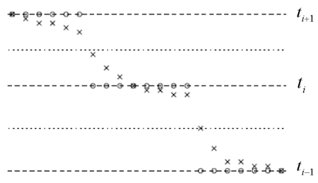
Figure 15: (cite?) The crosses show the values of \(f\), and the circles show the values of \(g\).
The theme of our proof is that if there is a large gap between \(\lambda_2\) and \(\lambda_k\), then the vector \(f\) in Lemma \ref{R1} can be well approximated by a \(2k+1\) step function. Let us start by the following lemma:
For any vector \(f\) such that \(\|f\|_w=1\), there exists a \((2k+1)\)-step approximation of \(f\), call \(g\), such that
\begin{equation} \nonumber \|f-g\|_w^2 \leq \frac{4 \mathcal{R}(f)}{\lambda_k}. \end{equation}\label{L1}
We want to find \(2k+1\) thresholds \(0=: t_0 \leq t_1 \leq \ldots \leq t_{2k}=M : = \max_v f(v)\) in a constructive manner. Let us define \(C:= 2 \mathcal{R}(f) /k\lambda_k\). The thresholds are chosen inductively. Given \(t_0, \ldots, t_{i-1}\), we define \(t_{i-1} \leq t_i \leq M\) to be the smallest number such that
\begin{equation} \sum_{v: t_{i-1} \leq f(v) \leq t_i} w(v) |f(v) - \psi_{t_{i-1},t_i}(f(v))|^2 = C, \label{eq1} \end{equation}and we put \(t_i =M\) if such number does not exist. Note that the LHS of \eqref{eq1} is a continuous function of \(t_i\), for \(t_i=t_{i-1}\) it is zero and when we keep increasing \(t_i\), the LHS does not decrease. We first prove that by this procedure \(t_{2k}=M\). By contradiction, assume that \(t_{2k} < M\). For \(1 \leq i \leq 2k\), let us define
\begin{eqnarray} \nonumber f_i(v):= \left \{\begin{array}{ll} |f(v) - \psi_{t_{i-1},t_i}(f(v))| & \text{if $t_{i-1} \leq f(v) \leq t_i$}, \\ 0 & \text{o.w.}\end{array} \right. \end{eqnarray}Clearly \(f_i\)'s are disjointly supported. We claim that for at least \(k\) of these functions we have \(\mathcal{R}(f_i) < \frac 12 \lambda_k\). Note that in the iterative procedure of choosing \(t_i\)'s we have \(t_i < M\) for all of them, so by \eqref{eq1} and the definition of \(f_i\)'s, we have \(\|f_i\|_w^2 =C\). We show that for any two vertices \(u\) and \(v\)
\begin{equation} \sum_{i=1}^{2k} |f_i(u)-f_i(v)|^2 \leq |f(u)-f(v)|^2. \label{eq2} \end{equation}
\(f_i\)'s are disjointly supported, so any two vertices \(u\) and \(v\) are in the support of at most two of these vectors. If both \(u\) and \(v\) are in the support of \(f_i\), then \eqref{eq2} is satisfied by equality. Otherwise, assume that \(u \in \text{supp}(f_i)\) and \(v \in \text{supp}(f_j)\) such that \(i
where the last inequality is from the fact that \(f(u) \leq t_i \leq t_{j-1} \leq f(v)\) by the above definitions. This completes the proof of \eqref{eq2}. Using the fact that \(\|f_i\|_w^2 =C\), we have
where in the last equation we used \(\|f\|_w=1\). This means that at least \(k\) of \(f_i\)'s must have a Rayleigh quotients less than \(\lambda_k /2\). This is a contradiction to Lemma \ref{R2}, so we must have \(t_{2k}=M\).
Let \(g\) be the \(2k+1\) step approximation of \(f\) using the derived thresholds. Using \eqref{eq1} we have:
In the above inequality, we used the fact that if \(t_i
Now we want to upper bound \(\phi(f)\) by using a \(2k+1\) step approximation of \(f\).
For any \((2k+1)\)-step approximation of \(f\) with \(\|f\|_w=1\) and \(\text{supp}(h) \leq vol(V) /2\), call \(g\),
\begin{equation} \nonumber \phi(f) \leq 4k \mathcal{R}(f) + 4\sqrt{2}k\|f-g\|_w \sqrt{\mathcal{R}(f)}. \end{equation}\label{P1}
Let \(g\) be a \(2k+1\) approximation of \(f\) with thresholds \(0 = t_0 \leq \ldots \leq t_{2k}\). Recall the definition of \(\phi(f)\) in \eqref{phi-f} that is the minimum of the conductance over all the threshold sets. This means that if two vectors \(f\) and \(h\) have the same threshold sets, they have the same conductances. Using this idea, instead of finding an upper bound on \(\phi(f)\), we find an upper bound on \(\phi(h)\) for another vector \(h\) with the same threshold sets as \(f\); so we have \(\phi(f) = \phi(h)\). Let us define a function \(\mu: \mathbb R \rightarrow \mathbb R\) as
\begin{equation} \nonumber \mu(x):= |x-\psi_{t_0,\ldots,t_{2k}} (x)|. \end{equation}Note that by the definition of \(g\) we have \(|f(v) - g(v)| = \mu(f(v))\). Now we define \(h\) as follows:
\begin{equation} \nonumber h(v):= \int_0^{f(v)} \mu(x) dx, \ \ \forall \ v \in V. \end{equation}First note that \(\mu(x)\) is a positive function, so \(h(u) \geq h(v)\) if and only if \(f(u) \geq f(v)\), which implies that \(h\) and \(f\) have the same threshold sets as we wanted. In view of Lemma \ref{R3}, our goal is to prove
\begin{equation} \nonumber \frac{\sum_{u \sim v} w(u,v) |h(u)-h(v)|}{\sum_vw(v) h(v)} \leq 4k \mathcal{R}(f) + 4\sqrt{2}k\|f-g\|_w \sqrt{\mathcal{R}(f)}. \end{equation}To do that, we try to bound the denominator and the numerator of the LHS separately in the following two claims.
Claim 1: For every vertex \(v\), we have
\begin{equation} \nonumber h(v) \geq \frac{1}{8k} f^2(v). \end{equation}To prove that, assume \(t_i < f(v) \leq t_{i+1}\), then by using Cauchy-Schwarz (C-S) inequality we have
\begin{eqnarray} f(v)^2 = \left(\sum_{j=0}^{i-1} (t_{j+1}-t_j)+(f(v) - t_i) \right)^2 & \leq & \left(\sum_{j=0}^{i-1} 1 \right) \left(\sum_{j=0}^{i-1} \left ((t_{j+1}-t_j)+(f(v) - t_i) \right)^2 \right), \ \ \ \text{(C-S)} \nonumber \\ &\leq& 2k \left(\sum_{j=0}^{i-1} (t_{j+1}-t_j)^2+(f(v) - t_i)^2 \right). \nonumber \end{eqnarray}The last inequality is by the fact that \(i \leq k\) and \((a+b)^2 \leq 2a^2+2b^2\) for any two real numbers. By definition of \(\mu(x)\), in the range \(t_j \leq x \leq t_{j+1}\), we have \(\mu(x) = x-t_j\) for \(t_j \leq x \leq (t_j+t_{j+1})/2\), and \(\mu(x) = t_{j+1}-x\) for \((t_j+t_{j+1})/2 \leq x \leq t_{j+1}\). Using the definition of \(h\) and the above simple fact, for every vertex \(v\) we can write:
\begin{eqnarray} h(v) &=& \sum_{j=0}^{i-1} \int_{t_j}^{t_{j+1}} \mu(x) dx + \int_{t_i}^{f(v)} \mu(x) dx = \sum_{j=0}^{i-1} \frac 14 (t_{j+1}-t_j)^2 + \int_{t_i}^{f(v)} \mu(x) dx \nonumber \\ & \geq& \sum_{j=0}^{i-1} \frac 14 (t_{j+1}-t_j)^2 + \int_{t_i}^{f(v)} (x-t_i) dx \geq \sum_{j=0}^{i-1} \frac 14 (t_{j+1}-t_j)^2 + \frac 14 (f(v)-t_i)^2, \nonumber \end{eqnarray}where we used the fact that \(t_i < f(v) \leq t_{i+1}\). Combining the above two inequalities, we get Claim 1.
Claim 2: For every pair of vertices \(u,v \in V\), we have
\begin{equation} \nonumber |h(v)-h(u)| \leq \frac 12 |f(v)-f(u)| \left (|f(u)-g(u)| + |f(v)-g(v)|+ |f(v)-f(u)| \right). \end{equation}To prove the claim, note that for any vertex \(v\) we have \(g(v)=\psi_{t_0,\ldots,t_{2k}} (f(v))\), hence by definition of \(\mu\), for any point \(f(v) < x \leq f(u)\), it is not difficult to see that \(\mu(x) \leq |x-g(u)|\) and \(\mu(x) \leq |x-g(v)|\). Using that, for any point \(f(v) < x \leq f(u)\), we have
\begin{eqnarray} \mu(x) &\leq& \min \{|x-g(u)|,|x-g(v)| \} \leq \frac{|x-g(u)|+|x-g(v)|}{2} \nonumber \\ &\leq & \frac 12 \left ( |x-f(u)| + |f(u)-g(u)| + |x - f(v)| + |f(v)-g(v)| \right), \ \ \text{triangle inequality}. \nonumber \\ &= & \frac 12 \left ( |f(v)-f(u)| + |f(u)-g(u)| + |f(v)-g(v)| \right). \nonumber \end{eqnarray}Therefore, we have
\begin{eqnarray} h(v)-h(u) = \int_{f(u)}^{f(v)} \mu(x) dx &\leq& |f(u)-f(v)| \max _{f(v) < x \leq f(u)} \mu(x) \nonumber \\ &\leq&\frac 12 |f(u) -f(v)| \left ( |f(v)-f(u)| + |f(u)-g(u)| + |f(v)-g(v)| \right), \nonumber \end{eqnarray}as we wanted.
Now by using Claim 2 and the fact that \(\|f\|_w^2=1\), we can write
\begin{eqnarray} &&\sum_{u \sim v} w(u,v) |h(u)-h(v)| \nonumber \\ &\leq& \sum_{u \sim v} \frac 12 w(u,v) |f(u) -f(v)| \left ( |f(v)-f(u)| + |f(u)-g(u)| + |f(v)-g(v)| \right) \nonumber \\ &\leq& \sum_{u \sim v} \frac 12 w(u,v) |f(u) -f(v)|^2 + \sum_{u \sim v} \frac 12 w(u,v) |f(u) -f(v)| \left ( |f(u)-g(u)| + |f(v)-g(v)| \right) \nonumber \\ &\underbrace{\leq}_{C-S}& \frac 12 \mathcal{R}(f) + \frac 12 \sqrt{ \sum_{u \sim v} w(u,v) |f(u) -f(v)|^2} \sqrt{ \sum_{u \sim v} w(u,v) \left ( |f(u)-g(u)| + |f(v)-g(v)| \right)^2} \nonumber \\ &\leq& \frac 12 \mathcal{R}(f) + \frac 12 \sqrt{ \mathcal{R}(f) } \sqrt{ 2\sum_{u \sim v} w(u,v) \left ( |f(u)-g(u)|^2 + |f(v)-g(v)|^2 \right)} \nonumber \\ &=& \frac 12 \mathcal{R}(f) + \frac 12 \sqrt{ \mathcal{R}(f) } \sqrt{ 2 \|f-g\|_w^2}. \nonumber \end{eqnarray}By using Claim 1, we can write
\begin{equation} \nonumber \sum_v w(v) h(v) \geq \frac{1}{8k} \sum_v w(v) f^2(v) = \frac{1}{8k} \|f\|_w^2 = \frac{1}{8k}. \end{equation}Putting together the above two inequalities, we get the statement of the proposition.
After proving Lemma \ref{L1} and Proposition \ref{P1}, the proof of the main theorem is immediate. Assume that \(f\) is a vector given by Lemma \ref{R1}, and let \(g\) be a vector given by Lemma \ref{L1}, then by using Proposition \ref{P1} we get
\begin{eqnarray} \phi(f) &\leq& 4k \mathcal{R}(f) + 4\sqrt{2}k\|f-g\|_w \sqrt{\mathcal{R}(f)} \ \ \ \text{(by Proposition \ref{P1})}\nonumber \\ &\leq& 4k \mathcal{R}(f) + 8\sqrt{2}k \mathcal{R}(f) / \sqrt{\lambda_k} \ \ \ \text{(by Lemma \ref{L1})} \nonumber \\ &\leq& 12\sqrt{2}k \mathcal{R}(f) / \sqrt{\lambda_k} \ \ \ \text{(using \(\lambda_k \leq 2\))}\nonumber \\ &\leq& 12\sqrt{2}k \frac{\lambda_2}{ \sqrt{\lambda_k}} \ \ \ \text{(by Lemma \ref{R1})}. \nonumber \end{eqnarray}This is the improved Cheeger's inequality.
10.4 Spectral algorithm for Max cut problem
In class, we saw Trevisan's spectral algorithm for finding the maximum cut in a graph with approximation guarantee slightly more than \(0.5\). In the same fashion as improved Cheeger's inequality, in this section, we see an improved bound using higher order spectral information. Using that, we introduce another max cut algorithm that actually uses higher order spectral information. Let us define the normalized sum Laplacian of a graph \(G\) as \(I + D^{-1/2}AD^{-1/2}\), with eigenvalues \(0 \leq \alpha_1 \leq \ldots \leq \alpha_n \leq 2\). Let \((L,R)\) be subset of vertices such that \(L \cup R \neq \emptyset\), then we define bipartiteness ratio of \((L,R)\) as:
\begin{equation} \nonumber \beta(L,R) := \frac{2w(E(L,L))+2w(E(R,R))+w(E(L \cup R,\overline{L \cup R}))}{vol(L \cup R)}. \end{equation}We define the bipartiteness ratio of a graph \(\beta(G)\) as the minimum of \(\beta(L,R)\) over all possible \((L,R)\). For a vector \(f\) and a threshold \(t\geq0\), let \(L_f(t):=\{v: f(v) \leq -t\}\) and \(R_f(t):=\{v: f(v) \geq t\}\) be a threshold cut of \(f\), then we define
\begin{equation} \nonumber \beta(f):= \min _{t \geq 0} \beta(L_f(t),R_f(t)), \end{equation}and we let \((L_f(t_{opt}),R_f(t_{opt}))\) be the best threshold set of \(f\). In this section, we abuse the definition of Rayleigh quotient of \(f\) as
\begin{equation} \nonumber \mathcal{R}(f):= \frac{\sum_{u \sim v}w(u,v)|f(u)+f(v)|^2}{\sum_v w(v) f(v)^2}. \end{equation}We proved the following lemma before
We also proved the following lemma that is very similar to the Cheeger's inequality and was the key point in designing the spectral max cut algorithm.
\label{L2}
Using Lemma \ref{L2}, we saw a spectral algorithm for the max cut problem that guarantees an approximation ratio more that \(0.5\). Similar to the idea used for Cheeger's inequality, if we can improve the upper bound in Lemma \ref{L2} be using higher order spectral information, we can improve the approximation guarantee. The improvement of Lemma \ref{L2}, in the same fashion as improved Cheeger's inequality, is the following theorem:
For any vector \(f\) and any \(1 \leq k \leq n\), we have
\begin{equation} \nonumber \beta(f) \leq 16\sqrt{2} k \frac{\mathcal{R}(f)}{\sqrt{\alpha_k}}, \end{equation}and by choosing \(f\) such that \(\mathcal{R}(f)=\alpha_1\) we get \(\beta(G) \leq O(k \alpha_1 / \sqrt{\alpha_k})\). \label{T2}
As can be seen, this theorem is very similar to improved Cheeger's inequality and the proof is also very similar. We can define a \(k\)-step approximation \(g\) of a vector \(f\) as before, the only difference is that here \(f\) can accept negative values. The proof of Theorem \ref{T2} follows from the following two lemmas that are the adaptation of Proposition \ref{P1} and Lemma \ref{L1}. We state them without proof as the proofs are similar to their counterparts.
For any vector \(f\) such that \(\|f\|_w^2 =1\), and \((2k+1)\)-step approximition \(g\) of that we have
\begin{equation} \nonumber \beta(f) \leq 4k \mathcal{R}(f) + 4\sqrt{2}k\|f-g\|_w \sqrt{\mathcal{R}(f)}. \end{equation}For any vector \(f\) such that \(\|f\|_w^2 =1\), at least one of the following holds
- \(\beta(f) \leq 8k \mathcal{R}(f)\).
- There exists \(k\) disjointly supported functions \(f_1,\ldots,f_k\) such that for all \(1 \leq i \leq k\) we have
\label{R4}
Note that we used Lemma \ref{L2} to prove the approximation guarantee for the Trevisan's max cut algorithm. Now that we have the improved bound of Theorem \ref{T2}, we can get a better bound for the same algorithm. However, we can do more and design an algorithm that uses higher order spectral information to get a better approximation bound.
The result proved in Trevisan's original paper \cite{tre} is stated slightly different from what we saw in class. The following theorem is the main result of \cite{tre}
Assume that the optimal solution of the max cut problem for a graph is \(1-\epsilon\). Given a parameter \(\delta\), there exists an algorithm that finds a vector \(h \in \{-1,0,1\}^V\) such that
\begin{equation} \nonumber \beta(h):= \frac{\sum_{u \sim v}w(u,v)|h(u)+h(v)|}{\sum_v w(v) |h(v)|} \leq 4 \sqrt{\epsilon}+\delta. \end{equation}\cite{tre} uses the above theorem to find a recursive algorithm with approximation guarantee of \(0.531\). The following theorem shows that by using higher order spectral information, a stronger result can be found.
Assume that the optimal solution of the max cut problem for a graph is \(1-\epsilon\). There exists a polynomial time algorithm that returns a cut \((S,\overline{S})\) that cuts
\begin{equation} \nonumber 1-O(k) \log\left( \frac{\alpha_k}{k \epsilon} \right)\frac{\epsilon}{\alpha_k} \end{equation}fraction of edges. \label{imp-cut}
In the rest of this paper, we state the algorithm and prove that if the algorithm works, we get the result of Theorem \ref{imp-cut}. To prove that the algorithm actually works and all the steps are consistent needs more work and an interested reader can find it in \cite{main}.
Let us define uncutness for a pair of cuts \((L,R)\) as follows
\begin{equation} \nonumber \gamma(L,R) := w(E(L,L))+w(E(R,R))+w(E(L \cup R, \overline{L \cup R})). \end{equation}Note that the coefficient of edges inside \(L\) and \(R\) is one instead of 2 in the definition of \(\beta(L,R)\). The edges that contribute to the uncutness are shown in Figure \ref{Fig4}.
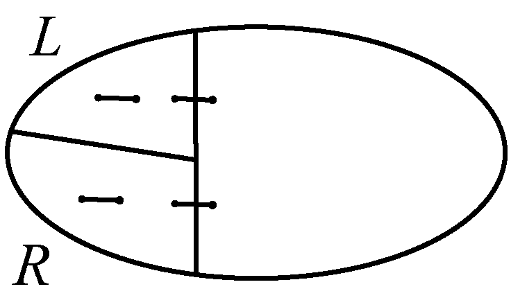
Figure 16: Edges that contribute to the uncutness.
Here is the algorithm \\
A spectral algorithm for max cut:
The algorithm maintains an induced cut \((L,R)\). To extend it, either we find an induced cut \((L',R')\) in the remaining graph \(H\) with \(\beta(H) = O(k \mathcal{R}_H(f) / \alpha_k)\), or we find an induced cut \((L',R')\) such that \\ \(\min(\gamma(L \cup L',R \cup R'),\gamma(L \cup R',R \cup L') ) \leq \gamma(L,R)\). In other words, we can extend our induced cut such that the uncutness does not increase. Let us see what it means not to increase the uncutness. Assume that \((L,R)\) is updated to \((L\cup L',R \cup R')\), then we have
\begin{equation} \nonumber \gamma(L \cup L',R \cup R') - \gamma(L,R) = - w(E(L,R'))-w(E(L',R))+ w(E(R'\cup L', \overline{ L\cup L' \cup R \cup R' })). \end{equation}All the edges we have in the RHS of the above equation are shown in Figure \ref{Fig5}. Not increasing the uncutness means that the weight of the edges cut in the \(j\)-th iteration (\(w(E(L,R'))+w(E(L',R))\)) is at least as large as the total weight of the edges removed from \(H\) in the \(j\)-th iteration (\(w(E(R'\cup L', \overline{L\cup L' \cup R \cup R'}))\)). This is important and shows that if \(\beta\) is not small, then we increase our cut at least as large as the edges we remove from \(H\).
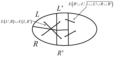
Figure 17: Edges that contribute to the difference of uncutness after one iteration of the second case of the algorithm.
We skip the proof that in the second case of the algorithm, we can always find \((L',R')\) with the desired properties, an interested reader can see the proof in \cite{main}. Assuming that, we now prove Theorem \ref{imp-cut}.
Assume that after a number of iterations \(U\) be the remaining vertices, and let \(H=(U,E(U))\) be the corresponding induced subgarph. Let \(\alpha'_1 \geq 0\) be the smallest eigenvalue of the sum Laplacian of \(H\). Also assume that \(w(E(U))= \rho w(E(V))\). We know that the optimal solution cuts at least \(1-\epsilon\) (weighted) fraction of edges of \(G\). This means that it must cut at least \(1- \epsilon /\rho\) fraction of the edges of \(H\), otherwise the total fraction of edges cut is less that \((1-\rho)+(1-\epsilon /\rho) \rho=1-\epsilon\), which is a contradiction. This means that for an eigenvector \(f\) of \(H\) with eigenvalue \(\alpha_1'\), using Lemma \ref{L2}, we have
\begin{equation} \nonumber \alpha'/2 \leq \beta(H) \leq \epsilon / \rho \ \Rightarrow \ \mathcal{R}_H(f) \leq 2\epsilon / \rho \end{equation}Using this, in the first case of the algorithm, we have
\begin{equation} \beta(L',R') \leq 192 \sqrt{2} k \mathcal{R}_H(f) / \alpha_k \leq 600k \frac{\epsilon}{\rho \alpha_k}. \label{eq3} \end{equation}Our goal is to find the ratio of the edges cut by the final solution of the algorithm. Let \(\rho_j w(E)\) be the fraction of edges in \(H\) before the \(j\)-th iteration of the while loop for all \(j \geq 1\), so we have \(\rho_1=1\). If the first case of the algorithm happens in iteration \(j\), then by using \eqref{eq3} we cut at least \((1-600k \frac{\epsilon}{\rho_j \alpha_k})\) fraction of edges removed from \(H\) in the \(j\)-th iteration. The weight of the edges before \((j+1)\)-th iteration is \(\rho_{j+1} w(E)\), so we can find the following bound on the weight of edges added to the cut at iteration \(j\)
\begin{equation} \nonumber (\rho_j-\rho_{j+1}) w(E) \left (1-600k \frac{\epsilon}{\rho_j \alpha_k} \right ) \geq w(E) \int_{\rho_{j+1}}^{\rho_{j}} \left (1-600k \frac{\epsilon}{r \alpha_k} \right ) dr. \end{equation}This inequality is by using the fact that \(\rho_j \geq \rho_{j+1}\) and the function in the integral is increasing.
In the second case of the algorithm, we choose a threshold cut of one of \(f_1,\ldots,f_k\). We choose \((L',R')\) such that the uncutness does not increase. As we explained above, this means that the weight of the edges cut in the \(j\)-th iteration is at least as large as the total weight of the edges removed from \(H\) in the \(j\)-th iteration. By our definition, this means the weight of the edges cut in the \(j\)-th iteration is at least \((\rho_j-\rho_{j+1}) w(E)\).
Assume that the \(j\)-th iteration is the last iteration that we use case 1 in the algorithm, then as we cut at least \((1-600k \frac{\epsilon}{\rho_j \alpha_k})\) of edges, we should have \(\rho_j \geq 600k \frac{\epsilon}{ \alpha_k}\). Using that and putting the above results for the two cases together, we conclude that the fraction of the edges cut by the algorithm is at least
\begin{equation} \nonumber \int_{600k \epsilon / \alpha_k} ^ 1\left (1-600k \frac{\epsilon}{r \alpha_k}\right ) dr = 1- \frac{600 k \epsilon}{ \alpha_k} \left ( 1+ \ln \left (\frac{\alpha_k}{600k \epsilon} \right )\right ). \end{equation}This completes the proof of Theorem \ref{imp-cut}.
10.5 Conclusion
In this paper, we introduced and proved the improved Cheeger's inequality that uses higher order spectral information to improve the upper bound on the conductance of a graph. We also saw how to find a similar result for the bipartiteness of a graph, and introduced an improved spectral algorithm for the max cut that uses higher order spectral information.
In the main reference \cite{main}, you can find a second proof for the improved Cheeger's inequality. As these proofs are constructive, each of them gives ideas for designing algorithms. Section 4 of \cite{main} is about the connections and applications, and we saw the max cut algorithm from that section. The other applications studied are spectral multiway partitioning, balanced separation, manifold setting, planted and semi-random instances, and stable instances.
11 An Almost-Linear-Time Algorithm for Approximate Max Flow in Undirected Graphs, and its Multicommodity Generalizations
This chapter is a summary of the paper "An Almost-Linear-Time Algorithm for Approximate Max Flow in Undirected Graphs, and its Multicommodity Generalizations," by Kelner et al. Unless noted otherwise, all results herein come from that paper. The main results are the existence of an \(O\left(m^{1 + o(1)}\epsilon^{-2}\right)\) algorithm for finding a \((1 - \epsilon)\)-approximate maximum flow and an \(O\left(m^{1 + o(1)}\epsilon^{-2}k^2\right)\) algorithm for finding a \((1 - \epsilon)\)-approximate maximum concurrent multicommodity flow on a capacitated, undirected graph, where \(m\) and \(k\) denote the number of edges and commodities, respectively.
We do not cover Sections 5 and 7 of the paper. The other sections are covered at varying levels of detail.
11.1 Resources
The paper is available at http://arxiv.org/abs/1304.2338, and a lecture by the first author is available at http://video.ias.edu/csdm/2014/0224-JonathanKelner.
11.2 Problem definition and main result
In this section, we formally state the Maximum Flow problem and the main result of the paper.
Let \(G = (V, E, \mu)\) be a capacitated graph. Throughout this report, all graphs are undirected. Let \(n = |V|\) and \(m = |E|\) denote the number of vertices and edges in \(G\), respectively. The vector \(\mu \in \left(\mathbb{R}_*^+\right)^E\) gives the capacities of the edges. We are also given a vector of vertex demands \(\chi \in \mathbb{R}^V\) satisfying \(\sum_{v \in V} \chi_v = 0\). Whenever we say that a vector is a vector of vertex demands, we assume that it has that property. Our goal is to find the maximum value of \(\alpha\) such that there exists a flow satisfying the vertex demands \(\alpha\chi\) and such that the amount of flow along each edge \(e \in E\) is at most its capacity \(\mu_e\).
Next, we introduce some notation to allow a more precise and concise statement of the problem. We assume an arbitrary orientation of the edges of \(E\), and we let \(f \in \mathbb{R}^E\) denote a flow. We denote by \(f_e\) the flow on an edge \(e = (u, v) \in E\). When \(f_e > 0\) (respectively, when \(f_e < 0\)), flow is being sent from vertex \(u\) to vertex \(v\) (respectively, from vertex \(v\) to vertex \(u\)). For a vertex \(v \in V\), we denote by \(\vec{1}_v \in \mathbb{R}^V\) the vector whose entry indexed by \(v\) is equal to one, and whose all other entries are equal to zero. We define the edge-vertex incidence matrix \(B \in \{-1, 0, 1\}^{E \times V}\), whose row indexed by an edge \(e = (u, v) \in E\) is equal to \(\left(\vec{1}_u - \vec{1}_v\right)^\intercal\). We let \(U \in \left(\mathbb{R}_*^+\right)^{E \times E}\) denote the diagonal matrix associated with the edge capacities.
Using the notation introduced, we can succinctly restate the problem as follows.
The Maximum Flow Problem: $$\label{MF1} \tag{MF$_1$} \max\left\{\alpha \in \mathbb{R} : \exists f \in \mathbb{R}^E \textrm{ such that } B^\intercal f = \alpha \chi \textrm{ and } \left\|U^{-1}f\right\|_{\infty} \le 1 \right\}$$
The following examples may help in understanding the notation. Figure 18 shows a graph \(G\) with $$B = \left( \begin{array}{cccc} 1 & -1 & 0 & 0 \\ 0 & 1 & -1 & 0 \\ 0 & 0 & -1 & 1 \\ 1 & 0 & 0 & -1 \\ \end{array} \right) \textrm{ and } U = \left( \begin{array}{cccc} 2 & 0 & 0 & 0 \\ 0 & 4 & 0 & 0 \\ 0 & 0 & 1 & 0 \\ 0 & 0 & 0 & 1 \\ \end{array} \right) \ .\notag$$
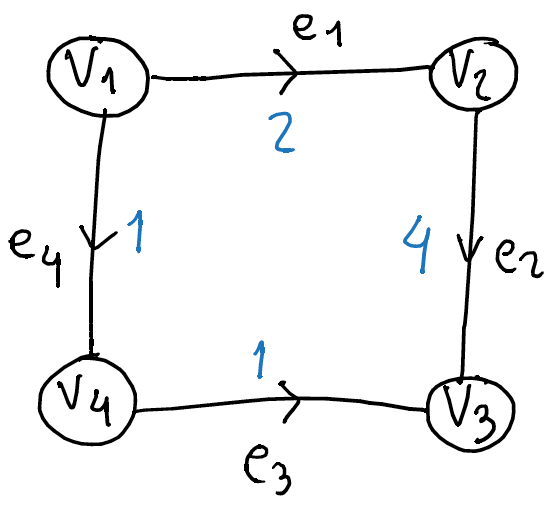
Figure 18: A sample graph \(G\). The blue numbers are the edge capacities, and the arrows represent the arbitrary orientation of the edges.
Figure 19 shows the flow \(f = \left(-3, -1, 1,-3\right)^\intercal\) on graph \(G\). Note that \(f\) satisfies the vector of vertex demands $$\begin{aligned}B^\intercal f & = & \left(\begin{array}{cccc} 1 & -1 & 0 & 0 \\ 0 & 1 & -1 & 0 \\ 0 & 0 & -1 & 1 \\ 1 & 0 & 0 & -1 \\ \end{array} \right)^{\intercal} \left(\begin{array}{c} -3\\ -1\\ 1\\ -3 \end{array}\right) = \left(\begin{array}{c} -6\\ 2\\ 0\\ 4\\ \end{array}\right)\ ,\end{aligned} \notag$$ and that \(f\) violates the capacity constraints, because $$\begin{aligned} \left\|U^{-1}f\right\|_{\infty}& = & \left( \begin{array}{cccc} 2 & 0 & 0 & 0 \\ 0 & 4 & 0 & 0 \\ 0 & 0 & 1 & 0 \\ 0 & 0 & 0 & 1 \\ \end{array} \right) ^{-1} \left( \begin{array}{c} -3 \\ -1 \\ 1 \\ -3 \\ \end{array} \right) = \left\|\left( \begin{array}{c} -\frac{3}{2} \\ - \frac{1}{4} \\ 1 \\ -3 \end{array}\right)\right\|_{\infty} = 3 > 1 \ .\end{aligned}\notag$$
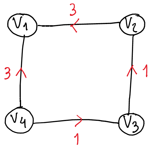
Figure 19: A sample flow \(f\) on graph \(G\). The number on each edge indicates the amount of flow going in the direction indicated by the arrow.
The main result of the paper is the following theorem. The capacity ratio of graph \(G\) is defined as the ratio between the maximum and the minimum capacity of an edge, and is denoted by \(S\).
If \(S = \textrm{poly}(n)\), then there exists an algorithm that finds a \((1 - \epsilon)\)-approximate maximum flow in time $$O\left(m2^{O\left(\sqrt{\log n \log \log n}\right)}\epsilon^{-2}\right) = O\left(m^{1 + o(1)}\epsilon^{-2}\right)\ . \label{theo:maxflow}$$
Prior to this paper, the most efficient algorithm known was due to Christiano et al, with running time $$\tilde{O}\left(mn^{\frac{1}{3}}\textrm{poly}\left(\epsilon^{-1}\right)\right) \ .\notag$$
11.3 Overview of the chapter
In Sections 11.5.1 – 11.5.3, we reformulate the Maximum Flow Problem \ref{MF1} as an unconstrained optimization problem. This reformulation requires the introduction of a projection matrix from the space of flows on \(G\) to the space of circulations on \(G\).
Section 11.5.5 describes how the Gradient Descent Method can be used to approximately solve the resulting unconstrained optimization problem. This requires replacing the objective function, which is non-differentiable, by a smooth approximation described in Section 11.5.4. Further, in order to avoid an inherent \(O(\sqrt{m})\) factor in the number of iterations, the authors introduce and analyze a non-Euclidean variant of the Gradient Descent Method, which is described in Section 11.4.
The running time of the algorithm presented in Section 11.5.5 depends heavily on the projection matrix used in the reformulation of the problem. Section 11.5.6 shows how to efficiently construct a projection matrix in order to obtain an almost-linear running time. Section 11.5.6.1 shows that this reduces to efficiently constructing an oblivious routing with low congestion, and Section 11.5.6.2 discusses how to construct such an oblivious routing. This is done by recursively constructing oblivious routings on smaller graphs. Obtaining a low-congestion oblivious routing for a graph from oblivious routings for smaller graphs is possible as long as there exist low-congestion embeddings from the original graph to the smaller ones and vice-versa. The recursive algorithm relies on two operations for obtaining smaller graphs: edge sparsification and vertex elimination. The former operation is based on Spielman and Teng and Spielman and Teng, while the latter is based on Madry, and presented on Section 11.5.6.3. The base case of the recursive algorithm uses electrical flows on graphs with \(O(1)\) vertices.
11.4 The Gradient Descent Method for general norms
In this section, we describe a method for solving the problem $$\label{P} \tag{P} \min_{y \in \mathbb{R}^n} f(y) \ ,$$ where \(f : \mathbb{R}^n \rightarrow \mathbb{R}\) is a convex function with Lipschitz-continuous gradient.
Let \(\|\cdot\| : \mathbb{R}^n \rightarrow \mathbb{R}\) be an arbitrary norm on \(\mathbb{R}^n\), and recall that the gradient of \(f\) at a point \(x \in \mathbb{R}^n\) is defined as being the vector \(\nabla f(x) \in \mathbb{R}^n\) such that $$f(y) = f(x) + \langle\nabla f(x), y - x\rangle + o\left(\left\|y - x\right\|\right) \ .\notag$$
The analysis of the Gradient Descent Method when \(\|\cdot\|\) is the \(\ell_2\)-norm relies on the Cauchy-Schwarz inequality to compare the improvement \(\langle\nabla f(x), y - x\rangle\) when moving from a point \(x\) to a point \(y\) with the step size \(\left\|y - x\right\|\) and the value \(\nabla f(x)\) of the gradient at \(x\). Here, we rely on an analogue of the Cauchy-Schwarz inequality. We introduce the dual norm \(\left\|\cdot\right\|^{*} : \mathbb{R}^n \rightarrow \mathbb{R}\), defined as follows: $$\left\|x\right\|^{*} = \max_{y \in \mathbb{R}^n : \left\|y\right\| \le 1} \langle y, x \rangle \ .\notag$$
For every \(x, y \in \mathbb{R}^n\), we have $$\label{cs} \langle y, x \rangle \le \left\|y\right\|^* \left\|x\right\|\ .$$
Bounding the convergence rate of the method requires assumptions on the smoothness of the gradient of \(f\). Specifically, we assume that \(\nabla f\) is Lipschitz-continuous with Lipschitz constant \(L \in \mathbb{R}^+\), that is, we assume that the following inequality holds for every two vectors \(x, y \in \mathbb{R}^n\): $$\left\|\nabla f(x) - \nabla f(y)\right\|^* \le L \left\|x - y\right\| \ .\notag$$
By integrating \(\frac{d}{dz}f(z)\) along a line going from \(z = x\) to \(z = y\), and using Lemma \ref{cs} and the Lipschitz-continuity of \(\nabla f\), one can prove the following result.
Let \(f : \mathbb{R}^n \rightarrow \mathbb{R}\) be a convex function with Lipschitz-continuous gradient with Lipschitz constant \(L\). Then for every \(x, y \in \mathbb{R}^n\) we have $$f(y) \le f(x) + \left \langle \nabla f(x), y - x\right \rangle + \frac{L}{2}\left\|x-y\right\|^2 \ .\label{la}$$
The Gradient Descent Method consists in choosing an initial point, and then at each iteration moving from the current point \(x\) to the point \(y\) that minimizes the upper bound on \(f(y)\) given by Lemma \ref{la}. If we let \(s = y - x\), then finding such a vector \(y\) amounts to solving
$$\min_{s \in \mathbb{R}^n} \left \langle \nabla f(x), s \right \rangle + \frac{L}{2} \left\|s\right\|^2 \ .\notag$$
By making the change of variable \(s = -\frac{s'}{L}\), one can show that the optimal step is \(s = -\frac{1}{L} \left(\nabla f(x)\right)^{\#}\), where $$\left(\nabla f(x)\right)^{\#} = \textrm{argmax}_{s \in \mathbb{R}^n} \langle \nabla f(x), s \rangle - \frac{1}{2}\|s\|^2 \ .\notag$$
We now state the Gradient Descent Method.
The Gradient Descent Method
- Choose a starting point \(x_0 \in \mathbb{R}^n\).
- For \(k \gets 0, 1, \dots\), until a stopping condition is met,
- let \(x_{k + 1} = x_k - \frac{1}{L} \left(\nabla f\left(x_k\right)\right)^{\#}\).
The following theorem bounds the convergence rate of the Gradient Descent Method. We let \(f^* \in \mathbb{R}\) be the optimal value of problem \ref{P} and \(X^* \subseteq \mathbb{R}^n\) be the set of optimal solutions, which we assume to be non-empty.
Let \(f : \mathbb{R}^n \rightarrow \mathbb{R}\) be a convex function with Lipschitz-continuous gradient with Lipschitz constant \(L\). Then for all \(k \in \mathbb{Z}_+\), we have $$f\left(x_k\right) - f^* \le \frac{2LR^2}{k + 4} \ ,\notag$$ where $$R = \max_{\substack{x \in \mathbb{R}^n \\ f(x) \le f\left(x_0\right)}} \min_{x^* \in X^*} \left\|x - x^*\right\| \ .\label{t_conv}$$
Note that the value of \(f\left(x_k\right)\) is non-increasing as \(k\) increases, as each iteration takes the optimal step with respect to the upper bound on \(f\) of Lemma \ref{la}, and the step \(s = 0\) is always a candidate. Thus, the parameter \(R\) is an upper bound on the distance between any point produced by the algorithm and its closest optimal solution.
11.5 Approximate Algorithm for the Maximum Flow Problem
In this section, we present an approximate algorithm for the Maximum Flow Problem using the Gradient Descent Method.
In Sections 11.5.1 – 11.5.3, we reformulate the problem as an unconstrained optimization problem, which requires introducing a circulation projection matrix. Figure 20 summarizes the steps of the reformulation. In Section 11.5.4, we introduce a smooth approximation of the objective function. In Section 11.5.5, we show how to apply the Gradient Descent Method to find an approximate solution, and we bound the running time of the algorithm. The running time will depend on properties of the projection matrix, and Section 11.5.6 discusses how to efficiently construct such a matrix with the desired properties.
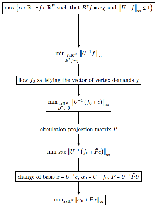
Figure 20: Reformulation of the Maximum Flow Problem as an unconstrained optimization problem.
11.5.1 Reformulation as Minimum Congestion Flow problem
Given a flow \(f \in \mathbb{R}^E\), we define the congestion of \(f\) to be the maximum ratio between the amount of flow through an edge (in absolute value) and its capacity, that is, $$\textrm{conge} (f) = \left\|U^{-1}f\right\|_{\infty} \ .\notag$$
Note that there exists a flow \(f\) satisfying vertex demands \(\alpha \chi\) and the edge capacities \(\mu\) if and only if there exists a flow satisfying vertex demands \(\chi\) with congestion at most \(\frac{1}{\alpha}\). Thus, the Maximum Flow Problem reduces to finding a flow satisfying vertex demands \(\chi\) with minimum congestion.
The Maximum Flow Problem – reformulation as Minimum Congestion Flow Problem $$\label{MF2} \tag{MF$_2$} \min_{\substack{f \in \mathbb{R}^E \\ B^\intercal f = \chi}} \left\|U^{-1}f\right\|_{\infty}$$
11.5.2 Reformulation as a circulation problem
Now, suppose that we are given a flow \(f_0 \in \mathbb{R}^E\) satisfying vertex demands \(\chi\). Note that \(f \in \mathbb{R}^E\) is a flow satisfying vertex demands \(\chi\) if and only if \(f - f_0 = c\) is a circulation. Thus, we can reformulate \ref{MF2} as follows.
The Maximum Flow Problem – reformulation as a circulation problem $$\tag{MF$_3$} \min_{\substack{c \in \mathbb{R}^E \\ B^\intercal c = \vec{0}}} \left\|U^{-1}\left(f_0 + c\right)\right\|_{\infty} \label{MF3}$$
11.5.3 Reformulation as an unconstrained problem
Note that \ref{MF3} is a constrained optimization problem. While the Gradient Descent Method can be adapted to constrained problems, this would require solving a constrained problem at each iteration. To avoid this, we can use a projection matrix to reformulate \ref{MF3} as an unconstrained problem.
A circulation projection matrix is a matrix \(\tilde{P} \in \mathbb{R}^{E \times E}\) such that:
- \(\tilde{P}\) maps every flow to a circulation, that is, \(B^\intercal\left(\tilde{P}x\right) = \vec{0}\) for all \(x \in \mathbb{R}^E\); and
- \(\tilde{P}\) maps every circulation to itself, that is, \(\tilde{P}x = x\) for all \(x \in \mathbb{R}^E\) such that \(B^\intercal x = \vec{0}\).
A circulation projection matrix \(\tilde{P}\) allows us to reformulate \ref{MF3} as follows: $$\min_{c \in \mathbb{R}^E} \left\|U^{-1}\left(f_0 + \tilde{P}c\right)\right\|_{\infty} \ .\notag$$
To further simplify the notation, we apply the change of basis \(x = U^{-1}c\), and we let \(\alpha_0 = U^{-1}f_0\) and \(P = U^{-1}\tilde{P}U\). We then get the following formulation, which will be used by the algorithm.
The Maximum Flow Problem – final reformulation $$\tag{MF$_4$} \min_{x \in \mathbb{R}^E} \left\|\alpha_0 + Px\right\|_{\infty} \label{MF4}$$
11.5.4 Approximating \(\|\cdot\|_\infty\) by a smooth function
The Gradient Descent Method as described in Section 11.4 cannot be directly applied to solve \ref{MF4}, because the objective function is not differentiable. Thus we introduce a smooth version of \(\|\cdot\|_{\infty}\), which we call \(\textrm{smax}_t\). For a parameter \(t \in \mathbb{R}^+\), we define \(\textrm{smax}_t : \mathbb{R}^E \rightarrow \mathbb{R}\) as follows: $$\textrm{smax}_t(x) = t \ln \left(\frac{\sum_{e \in E}e^{\frac{x_e}{t}} + e^{-\frac{x_e}{t}}}{2m}\right) \ .\notag$$
We will need three key properties of \(\textrm{smax}_t\): it approximates \(\|\cdot\|_{\infty}\), it is convex and it is smooth. The following lemma quantifies these properties.
The function \(\textrm{smax}_t\) satisfies the following inequality for every vector \(x \in \mathbb{R}^E\): $$\left\|x\right\|_{\infty} - t \ln (2m) \le \textrm{smax}_t(x) \le \left\|x\right\|_{\infty} \ .\notag$$ Moreover, \(\textrm{smax}_t\) is convex and has a Lipschitz-continuous gradient with Lipschitz constant $$\frac{1}{t}\label{l_smax}$$.
We prove only the first part of the statement. Note that $$0 \le e^{\frac{x_e}{t}} \le e^{\frac{\left\|x\right\|_{\infty}}{t}}\notag$$ and $$0 \le e^{-\frac{x_e}{t}} \le e^{\frac{\left\|x\right\|_{\infty}}{t}} \ ,\notag$$ for all \(e \in E\). Moreover, we have $$e^{\frac{\left\|x\right\|_{\infty}}{t}} = \max_{e \in E} \max\left\{e^{\frac{x_e}{t}}, e^{-\frac{x_e}{t}}\right\}\notag$$
Thus we get $$\begin{aligned} t \ln \left(\frac{\sum_{e \in E}e^{\frac{x_e}{t}} + e^{-\frac{x_e}{t}}}{2m}\right) & \ge & t \ln \left(\frac{e^{\frac{\left\|x\right\|_{\infty}}{t}}}{2m} \right) \\ & = & \left\|x\right\|_{\infty} - t \ln (2m) \end{aligned}\notag$$ and $$\begin{aligned} t \ln \left(\frac{\sum_{e \in E}e^{\frac{x_e}{t}} + e^{-\frac{x_e}{t}}}{2m}\right) & \le & t \ln \left(\frac{2m e^{\frac{\left\|x\right\|_{\infty}}{t}}}{2m} \right) \\ & = & \left\|x\right\|_{\infty} \ . \end{aligned}\notag$$
11.5.5 Solving the Maximum Flow Problem using the Gradient Descent Method
In this section, we show how the Gradient Descent Method can be used to approximately solve the Maximum Flow Problem.
Let \(f_0\) be an initial flow satisfying vertex demands \(\chi\), and let \(\textrm{OPT}\) be the minimum congestion of a flow satisfying vertex demands \(\chi\), that is, the optimal value of \ref{MF4}. The algorithm is stated below.
Approximate Maximum Flow algorithm
- Let \(\alpha_0 = U^{-1}f_0\), \(x_0 = -\alpha_0\).
- Let \(\left\|\cdot\right\| = \left\|\cdot\right\|_{\infty}\), \(t = \frac{\epsilon\textrm{OPT}}{2\ln (2m)}\) and \(k = \frac{300\left\|P\right\|_{\infty}^4\ln(2m)}{\epsilon^2}\).
- Let \(g_t = \textrm{smax}_t \left(\alpha_0 + Px\right)\).
- For \(i = 0, \dots, k - 1\), do
- let \(x_{i + 1} = x_i - \frac{t}{\left\|P\right\|_{\infty}^2} \left(\nabla g_t(x_i)\right)^{\#}\).
- Let \(f = U\left(\alpha_0 + Px_k\right)\).
- Output \(\frac{f}{\textrm{conge}(f)}\).
In step 1, we initialize \(\alpha_0\) according to the definition given in the reformulation leading from to \ref{MF3} to \ref{MF4}, and we define the initial point \(x_0\) (the choice of \(x_0\) will play a role in bounding the value of \(R\)). In step 2, we set three parameters for the Gradient Descent Method, namely the norm \(\|\cdot\|\), the parameter \(t\) used for smoothing the objective function, and the number of iterations \(k\). Step 3 introduces a smooth function \(g_t\) that approximates the objective function of . We will call \(g_t\) the approximate objective function, and \(\left\|\alpha_0 + Px\right\|_{\infty}\) the exact objective function. Steps 4 – 5 use the Gradient Descent Method to solve the problem
$$\tag{MF$_4'$} \min_{x \in \mathbb{R}^E} g_t(x) \ , \label{MF4b}$$
which is obtained from \ref{MF4} by replacing the exact objective function by the approximate objective function. Steps 6 and 7 correspond to undoing the operations used in reformulating \ref{MF1} as \ref{MF4}: note that $$\begin{aligned} f & = & f_0 + \tilde{P}c \\ & = & U\left(U^{-1}f_0 + U^{-1}\tilde{P}c\right)\\ & = & U\left(\underbrace{U^{-1}f_0}_{\alpha_0} + \underbrace{U^{-1}\tilde{P}U}_{P}x\right) \\ & = & U\left(\alpha_0 + Px\right) \ , \end{aligned}\notag$$ and that dividing \(f\) by \(\textrm{conge}(f)\) corresponds to scaling the flow \(f\) by the largest possible factor without violating the edge capacity constraints.
Before presenting the analysis of the algorithm, let us make two remarks concerning the implementation. The algorithm requires as input a flow \(f_0\) satisfying vertex demands \(\chi\). This can be obtained in almost-linear time using electrical flows. Moreover, it requires as input \(\textrm{OPT}\), that is, the optimal value of \ref{MF4}. Note that we can approximate \(\textrm{OPT}\) using binary search.
We now proceed to the analysis of the algorithm, which will justify the choice of the parameters \(t\) and \(k\). For a matrix \(A\), we denote by \(\mathcal{T}(A)\) the time needed to multiply a vector by \(A\) or \(A^\intercal\). Note that the matrices we will use will not be represented explicitely. Instead, when analyzing the running time, we will think of a matrix \(A\) as being a linear function, and of \(\mathcal{T}(A)\) as being the time needed to evaluate it at a vector.
The algorithm described outputs a (\(1 - O(\epsilon)\))-approximate maximum flow in time $$O\left(\|P\|_{\infty}^4 \log m (\mathcal{T}(P) + m)\epsilon^{-2}\right) \ .\notag$$
The proof relies on Theorem \ref{t_conv}. Using the fact that the gradient of \(\textrm{smax}_t\) is Lipschitz-continuous with Lipschitz constant \(\frac{1}{t}\) (see Lemma \ref{l_smax}), one can show that the gradient of \(g_t\) is Lipschitz-continuous with Lipschitz constant \(L = \frac{\|P\|_{\infty}^2}{t}\).
Now, we need to bound the value of \(R\). Recall that the parameter \(R\) is equal to the maximum distance between a point \(x \in \mathbb{R}^E\) such that \(g_t(x) \le g_t\left(x_0\right)\) and its nearest optimal solution to \ref{MF4}. Let \(X^*\) denote the set of optimal solutions to \ref{MF4}, and \(\textrm{OPT}'\) denote the optimal value. Lemma \ref{l_smax} clearly implies that \(\textrm{OPT}' \le \textrm{OPT}\).
In order to bound that distance for such a point \(x\), we will construct an optimal solution whose distance to \(x\) is small. Specifically, given an optimal solution \(y^* \in X^*\), we claim that \(x - Px + Py^*\) is also an optimal solution and that it is close to \(x\). Note that, since \(\tilde{P}\) is a projection matrix, we have \(\tilde{P}^2 = \tilde{P}\). Note that \(P\) has the same property: we have $$\begin{aligned} P^2 & = & \left(U^{-1}\tilde{P}U\right)\left(U^{-1}\tilde{P}U\right) \\ & = & U^{-1}\tilde{P}^2U \\ & = & U^{-1}\tilde{P}U \\ & = & P \ . \end{aligned}\notag$$ Thus we have $$\begin{aligned} P(x - Px + Py^*) & = & Px - P^2x + P^2y^* \\ & = & Py^* \ . \end{aligned}\notag$$ It follows that the approximate objective function attains the same value at \(y^*\) and \(x - Px + Py^*\), and therefore \(x - Px + Py^* \in X^*\).
Using that fact, we can upper bound \(R\) as follows: $$\begin{aligned} \label{eqa} R & = & \max_{\substack{x \in \mathbb{R}^E \\ g_t(x) \le g_t\left(x_0\right)}} \min_{x^* \in X^*} \left\|x - x^*\right\|_{\infty} \notag\\ & \le & \max_{\substack{x \in \mathbb{R}^E \\ g_t(x) \le g_t\left(x_0\right)}} \left\|x - \left(x - Px + Py^*\right)\right\|_{\infty} \notag\\ & = & \max_{\substack{x \in \mathbb{R}^E \\ g_t(x) \le g_t\left(x_0\right)}} \left\|Px - Py^*\right\|_{\infty}\notag \\ & = & \max_{\substack{x \in \mathbb{R}^E \\ g_t(x) \le g_t\left(x_0\right)}} \left\|\alpha_0 + Px - \alpha_0 - Py^*\right\|_{\infty} \notag\\ & \le & \max_{\substack{x \in \mathbb{R}^E \\ g_t(x) \le g_t\left(x_0\right)}} \left\|\alpha_0 + Px\right\|_{\infty} + \left\| \alpha_0 + Py^*\right\|_{\infty} \notag\\ & \le & g_t(y^*) + t\ln(2m) + \max_{\substack{x \in \mathbb{R}^E \\ g_t(x) \le g_t\left(x_0\right)}} \left\|\alpha_0 + Px\right\|_{\infty} \notag\\ & = & \textrm{OPT}\phantom{}' + t\ln(2m) + \max_{\substack{x \in \mathbb{R}^E \\ g_t(x) \le g_t\left(x_0\right)}} \left\|\alpha_0 + Px\right\|_{\infty}\notag \\ & \le & \textrm{OPT} + t\ln(2m) + \max_{\substack{x \in \mathbb{R}^E \\ g_t(x) \le g_t\left(x_0\right)}} \left\|\alpha_0 + Px\right\|_{\infty} \ . %& \le & \textrm{OPT} + \left(1 + \|P\|_{\infty}\right) \textrm{OPT} + t \ln(2m) \\ %& = & \left(2 + \|P\|_{\infty}\right) \textrm{OPT} + t \ln(2m) \ . \end{aligned}$$
Now, we need to bound the value of the exact objective function at a point \(x \in \mathbb{R}^E\) such that \(g_t(x) \le g_t(x_0)\). Lemma \ref{l_smax} allows us to bound that value with respect to the value at \(x_0\): we have $$\begin{aligned} \label{eqb} \left\|\alpha_0 + Px\right\|_{\infty} & \le & g_t(x) + t\ln(2m) \notag\\ & \le & g_t(x_0) + t\ln(2m) \notag\\ & \le & \left\|\alpha_0 + Px_0\right\|_{\infty} + t\ln(2m) \ . \end{aligned}$$
Now it suffices to bound the value of the exact objective function at the initial point \(x_0\). Let \(z^*\) be an optimal solution to \ref{MF4} such that \(Pz^* = z^*\). Such a solution exists because, if \(c^*\) is an optimal solution to \ref{MF3}, then clearly \(z^* = U^{-1}c^*\) is an optimal solution to \ref{MF4}, and we have $$\begin{aligned} P\left(U^{-1}c^*\right) & = & U^{-1}\tilde{P}UU^{-1}c^* \\ & = & U^{-1}\tilde{P}c^* \\ & = & U^{-1}c^* \ . \end{aligned}\notag$$ Using that optimal solution \(z^*\), we get $$\begin{aligned} \label{eqc} \left\|\alpha_0 + Px_0\right\|_{\infty} & = & \left\|\alpha_0 - P\alpha_0 \right\|_{\infty} \notag\\ & = & \left\|\alpha_0 + Pz^* - Pz^* - P\alpha_0 \right\|_{\infty} \notag\\ & \le & \left\|\alpha_0 + Pz^* \right\|_{\infty} + \left\|Pz^* + P\alpha_0 \right\|_{\infty} \notag\\ & = & \left\|\alpha_0 +Pz^* \right\|_{\infty} + \left\|P\left( \alpha_0 + z^*\right) \right\|_{\infty} \notag\\ & = & \left\|\alpha_0 +Pz^* \right\|_{\infty} + \left\|P\left( \alpha_0 + Pz^*\right) \right\|_{\infty}\notag \\ & \le & \left(1 + \|P\|_{\infty}\right) \left\|\alpha_0 + Pz^* \right\|_{\infty}\notag \\ & = & \left(1 + \|P\|_{\infty}\right) \textrm{OPT} \ . \end{aligned}$$
Combining inequalities \ref{eqa} – \ref{eqc} yields $$\begin{aligned} R & \le & \textrm{OPT} + t\ln(2m) + \max_{\substack{x \in \mathbb{R}^E \\ g_t(x) \le g_t\left(x_0\right)}} \left\|\alpha_0 + Px\right\|_{\infty} \\ & \le & \textrm{OPT} + t\ln(2m)+ \left\|\alpha_0 + Px_0\right\|_{\infty} + t\ln(2m) \\ & \le & \left(2 + \|P\|_{\infty}\right) \textrm{OPT} + 2t \ln(2m) \ . \end{aligned}\notag$$
Now that we have upper bounds on the parameters \(L\) and \(R\), we can apply Theorem \ref{t_conv} to bound the value of the approximate objective function at the final vector \(x_k\): we have $$\begin{aligned} g_t\left(x_k\right) & \le & \textrm{OPT}\phantom{}' + \frac{2LR^2}{k + 4} \\ & \le & \textrm{OPT} + \frac{2LR^2}{k + 4} \ . \end{aligned}\notag$$
Lemma \ref{l_smax} allows us to bound the value of the exact objective function at \(x_k\): we have $$\begin{aligned} \left\|\alpha_0 + Px_k\right\|_{\infty} & \le & g_t\left(x_k\right) + t\ln(2m) \\ & \le & \textrm{OPT} + \frac{2LR^2}{k + 4} + t\ln(2m) \ . \end{aligned}\notag$$
Plugging in the values of \(t\) and \(k\) and using the upper bounds on \(L\) and \(R\) yields $$\left\|\alpha_0 + Px_k\right\|_{\infty} \le (1 + \epsilon) \textrm{OPT} \ .\notag$$ Thus the algorithm returns a flow whose congestion is within \(1 + \epsilon\) of the minimum congestion, and hence a flow whose value \(\alpha\) is within \(\frac{1}{1 + \epsilon} = 1 - O(\epsilon)\) of the optimal value of \ref{MF1}.
Note that the running time is dominated by step 5. One can show that the expression for \(x_{i + 1}\) can be evaluated in time \(O (\mathcal{T}(P) + m)\), by showing that for every vector \(z \in \mathbb{R}^E\) and for every edge \(e \in E\), we have $$\left(\nabla z ^{\#}\right)_e = \textrm{sign} (z_e) \|z\|_1 \ .\notag$$ Multiplying by \(k\) yields the desired running time.
11.5.6 Constructing a projection matrix
In Section 11.5.5, we showed how to find a (\(1 - O(\epsilon)\))-approximate maximum flow in time $$O\left(\|P\|_{\infty}^4 \log m (\mathcal{T}(P) + m)\epsilon^{-2}\right) \ .\notag$$ In order to attain the desired running time for Theorem \ref{theo:maxflow}, namely $$O\left(m^{1 + o(1)}\epsilon^{-2}\right) \ ,\notag$$ we need to be able to efficiently construct a projection matrix \(\tilde{P}\) and the matrix \(P = U^{-1}\tilde{P}U\) in such a way that we can bound \(\|P\|_{\infty}\) and \(\mathcal{T}(P)\) appropriately.
11.5.6.1 Reduction to oblivious routing
In this section, we show that finding an appropriate projection matrix \(\tilde{P}\) reduces to finding an oblivious routing with low congestion.
A (linear) oblivious routing on a graph \(G = (V, E)\) is a matrix \(A \in \mathbb{R}^{E \times V}\) such that \(B^\intercal A\chi = \chi\) for all vectors of vertex demands \(\chi \in \mathbb{R}^V\). Note that the relation \(B^\intercal A\chi = \chi\) states that \(A\chi\) is a flow satisfying vertex demands \(\chi\).
Given a set of \(k\) vectors of vertex demands \(D = \left\{\chi^i\right\}_{i \in [k]}\), one can use an oblivious routing \(A\) to route each vector of vertex demands \(\chi^i\) individually using a flow \(f^i = A\chi^i\), obliviously to the existence of the other demands. The congestion of a set of flows \(\left\{f^i\right\}_{i \in [k]}\) is defined as follows: $$\begin{aligned} \textrm{conge}\left(\left\{f^i\right\}_{i \in [k]}\right) = \textrm{conge}\left(\sum_{i \in [k]}\left|f^i\right|\right) \ . \end{aligned}\notag$$
Figure 21 illustrates this definition. We have $$\begin{aligned} \textrm{conge}\left(\left\{f^1, f^1\right\}\right) & = & \textrm{conge}(f^3) \\ & = & 4 \ . \end{aligned}\notag$$ Note that the \(k\) flows do not cancel each other out over an edge, even if they go in opposite directions.
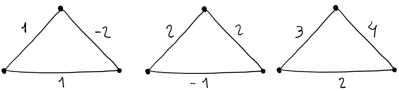
Figure 21: Three flows \(f^1\) (left), \(f^2\) (middle), and \(f^3 = \left|f^1\right| + \left|f^2\right|\) (right) in a graph with unit edge capacities.
The optimal congestion for routing the demands \(D\) is $$\textrm{OPT}\left(D\right) = \min_{\substack{\left\{f^i\right\}_{i \in [k]} \\ f^i \in \mathbb{R}^E, B^\intercal f^i = \chi^i \textrm{ for all } i \in [k]}} \textrm{conge} \left(\left\{f^i\right\}_{i \in [k]}\right) \ .\notag$$
The competitive ratio of an oblivious routing \(A\) is defined as being the maximum ratio between the congestion obtained by routing a set of finitely many demands obliviously and by routing them optimally:
$$\label{def_rho} \rho(A) = \max_{\substack{\{\chi^i\}_{i \in [k]} \\ \chi^i \in \mathbb{R}^V, \sum_{v \in V}\chi^i_v = 0 \textrm{ for all } i \in [k]}} \frac{\textrm{conge}\left(\left\{A\chi^i\right\}_{i \in [k]}\right)}{\textrm{OPT}\left(\left\{\chi^i\right\}_{i \in [k]}\right)} \ .$$
The following lemma shows that we can express the competitive ratio of an oblivious routing using simple matrix operations.
If \(A\) is an oblivious routing, then $$\rho(A) = \left\|U^{-1}AB^\intercal U\right\|_{\infty} .\label{lemma_cr}$$
We give a more detailed proof than the one in the paper.
Let \(\mathcal{D}\) denote the set of all possible sets of vectors of vertex demands, that is, the set of all finite, non-empty subsets of \(\left\{\chi \in \mathbb{R}^V : \sum_{v \in V} \chi_v = 0 \right\}\).
Given a set of vertex demands \(D \in \mathcal{D}\), let \(\left\{f^\chi\right\}_{\chi \in D}\) be the optimal routing of \(D\). Now, consider the set of demands \(D' = \left\{\chi'^e\right\}_{e \in E}\), in which, for each edge \((u, v) \in E\), we have a demand \(\chi'^e = F_e \left(\vec{1}_u - \vec{1}_v\right)\), where \(F = \sum_{\chi \in D} \left|f^\chi\right|\) is a vector giving the total amount of flow along each edge in the optimal routing of \(D\). Let \(\mathcal{D}'\) be the set of all sets of demands which can be obtained in this way, that is, let $$\mathcal{D}' = \left\{D' : D \in \mathcal{D}\right\} \ .\notag$$
We claim that, in Equation \ref{def_rho}, which defines the competitive ratio \(\rho(A)\), the maximum is attained by a demand \(D' \in \mathcal{D}'\). We can prove this by showing that the ratio obtained for \(D'\) is always larger than the ratio obtained for \(D\), that is, for every \(D \in \mathcal{D}\), we have $$\label{eq_ratios} \frac{\textrm{conge}(\left\{A\chi\right\}_{\chi \in D})}{\textrm{OPT}\left(D\right)} \le \frac{\textrm{conge}\left(\left\{A\chi'\right\}_{\chi' \in D'}\right)}{\textrm{OPT}\left( D'\right)}$$
First, note that $$\label{eq_den} \textrm{OPT}(D) \ge \textrm{OPT}\left(D'\right) \ ,$$ as we can satisfy each demand \(\chi'^e \in D'\) by the flow \(F_e \left(\vec{1}_u - \vec{1}_v\right)\), which yields a congestion equal to \(\textrm{OPT}(D)\).
Next, we show that $$\label{eq_num} \textrm{conge}(\left\{A\chi\right\}_{\chi \in D}) \le \textrm{conge}(\left\{A\chi'\right\}_{\chi' \in D'}) \ .$$
Note that the vector \(f^D \in \left(\mathbb{R_+}\right)^E\) giving the total flow along each edge when we obliviously route the set of demands \(D\) is $$\begin{aligned} f^D & = & \sum_{\chi \in D} \left|A\chi\right| \\ & = & \sum_{\chi \in D} \left|A\left(B^\intercal f^{\chi}\right)\right| \\ & = & \sum_{\chi \in D} \left|A \left(\sum_{e = (u,v) \in E} f^\chi_e \left(\vec{1}_u - \vec{1}_v\right)\right)\right| \\ & = & \sum_{\chi \in D} \left|\sum_{e = (u,v) \in E} f^\chi_e \left(A \left(\vec{1}_u - \vec{1}_v\right)\right)\right| \\ & \le & \sum_{\chi \in D} \sum_{e = (u,v) \in E} \left|f^\chi_e A \left(\vec{1}_u - \vec{1}_v\right)\right| \\ & = & \sum_{e = (u,v) \in E} \underbrace{\sum_{\chi \in D} \left|f^\chi_e\right|}_{F_e} \left|A \left(\vec{1}_u - \vec{1}_v\right)\right| \\ & = & \sum_{e = (u,v) \in E} F_e \left| A \left(\vec{1}_u - \vec{1}_v\right)\right| \ . \end{aligned}\notag$$
On the other hand, the vector \(f^{D'} \in \left(\mathbb{R_+}\right)^E\) giving the total flow along each edge when we obliviously route the set of demands \(D'\) is $$\begin{aligned} f^{D'} & = & \sum_{e \in E} \left|A\chi'^e\right| \\ & = & \sum_{e = (u,v)\in E} \left|A\left(F_e\left(\vec{1}_u - \vec{1}_v\right)\right)\right| \\ & = & \sum_{e = (u, v) \in E} F_e \left| A \left(\vec{1}_u - \vec{1}_v\right) \right| \ . \end{aligned}\notag$$ Thus we get \(f^D \le f^{D'}\), which implies \ref{eq_num}.
Combining \ref{eq_den} and \ref{eq_num} yields \ref{eq_ratios}. Thus we have $$\begin{aligned} \label{max_over_dp} \rho(A) & = & \max_{D \in \mathcal{D}} \frac{\textrm{conge}\left(\left\{A\chi\right\}_{\chi \in D}\right)}{\textrm{OPT}\left(D\right)} \notag \\ & = & \max_{D' \in \mathcal{D}'} \frac{\textrm{conge}\left(\left\{A\chi'\right\}_{\chi' \in D'}\right)}{\textrm{OPT}\left(D'\right)} \ . \end{aligned}$$
Now, we argue that $$\label{eq_den_rev} \textrm{OPT}(D) \le \textrm{OPT}\left(D'\right) \ .$$ Indeed, given a set of flows \(\left\{g^e\right\}_{e \in E}\) satisfying the set of demands \(D' = \left\{\chi'^e\right\}_{e \in E}\), one can obtain a set of flows \(\left\{h^\chi\right\}_{\chi \in D}\) satisfying the set of demands \(D\) without increasing the congestion, that is, with $$\label{dec_conge} \textrm{conge}\left(\left\{h^\chi\right\}_{\chi \in D}\right)\le \textrm{conge} \left( \left\{g^e\right\}_{e \in E}\right) \ .$$ To do this, we can start with the optimal routing \(\left\{f^\chi\right\}_{\chi \in D}\) for the set of demands \(D\). Then, for each edge \(e \in E\) and each demand \(\chi \in D\) at a time, we reroute the \(f^\chi_e\) units of flow along edge \(e\) by using the flow \(f^\chi_e \frac{g^e}{F_e}\). After doing this, we have that the vector giving the total amount of flow along each edge in the routing \(\left\{h^\chi\right\}_{\chi \in D}\) of the set of demands \(D\) is $$\begin{aligned} \sum_{\chi \in D} \left|h^\chi\right| & = &\sum_{\chi \in D} \left| \sum_{e \in E } f^\chi_e \frac{g^e}{F_e} \right| \\ & \le & \sum_{\chi \in D} \sum_{e \in E } \left| f^\chi_e \frac{g^e}{F_e} \right| \\ & = & \sum_{\chi \in D} \sum_{e \in E } \left| \frac{f^\chi_e}{F_e} \right| \left|g^e\right| \\ & = & \sum_{e \in E} \underbrace{\left(\sum_{\chi \in D} \left| \frac{f^\chi_e}{F_e} \right|\right)}_{1} \left|g^e\right| \\ & = & \sum_{e \in E} \left|g^e\right| \ , \end{aligned}\notag$$ which implies \ref{dec_conge}.
Now, \ref{eq_den} and \ref{eq_den_rev} yield $$\begin{aligned} \textrm{OPT}\left(D'\right) & = & \textrm{OPT}(D) \\ & = & \left\|U^{-1}F\right\|_{\infty} \ . \end{aligned}$$
We would like to replace the maximization over demands \(D' \in \mathcal{D}'\) in \ref{max_over_dp} to a maximization over arbitrary vectors \(x \in \mathbb{R}^E \setminus \{\vec{0}\}\). However, it is not obvious how to express \(\textrm{OPT}\left(\tilde{D}(x)\right)\), where \(x \in \mathbb{R}^E \setminus \{\vec{0}\}\) is an arbitrary vector and \(\tilde{D}(x) = \left\{x_e \left(\vec{1}_u - \vec{1}_v\right)\right\}_{e = (u, v) \in E}\). Nonetheless, it is easy to bound it: since we could route the demand \(x_e \left(\vec{1}_u - \vec{1}_v\right)\) through edge \(e\) for all edges \(e \in E\), we have $$\label{bound_opt} \textrm{OPT}\left( \tilde{D}\right) \le \left\| U^{-1}x \right\|_{\infty} \ .$$
We claim that the following equation holds: $$\begin{aligned} \label{rho_arb} \rho(A) & = & \max_{x \in \mathbb{R}^E \setminus \{\vec{0}\}} \frac{\textrm{conge}\left(\left\{A\chi\right\}_{\chi \in \tilde{D}(x)}\right)}{\left\|U^{-1} x\right\|_{\infty}} \ . \end{aligned}$$
Consider a vector \(x \in \mathbb{R}^E \setminus \{\vec{0}\}\). If \(\tilde{D}(x) \in \mathcal{D}'\), then the ratio we have in \ref{rho_arb} is equal to the ratio that we had in \ref{max_over_dp}. If \(\tilde{D}(x) \not \in \mathcal{D}'\), then using \ref{bound_opt}, we have that the ratio appearing in \ref{rho_arb} is $$\frac{\textrm{conge}\left(\left\{A\chi\right\}_{\chi \in \tilde{D}(x)}\right)}{\left\|U^{-1} x\right\|_{\infty}} \le \frac{\textrm{conge}\left(\left\{A\chi\right\}_{\chi \in \tilde{D}(x)}\right)}{\textrm{OPT}\left(\tilde{D}(x)\right)} \\ \le \rho(A) \ ,\notag$$ where the last step uses the fact that the ratio $$\frac{\textrm{conge}\left(\left\{A\chi\right\}_{\chi \in \tilde{D}(x)}\right)}{\textrm{OPT}\left(\tilde{D}(x)\right)}\notag$$ was one of the candidates in \ref{def_rho}. Thus these extraneous terms are not a problem, and it follows that \ref{rho_arb} is equivalent to \ref{max_over_dp}. Using \ref{rho_arb}, we get $$\begin{aligned} \label{exp_rho} \rho(A) & = & \max_{x \in \mathbb{R}^E \setminus \{\vec{0}\}} \frac{\textrm{conge}\left(\left\{A\chi\right\}_{\chi \in \tilde{D}(x)}\right)}{\left\|U^{-1} x\right\|_{\infty}} \\ & = & \max_{x \in \mathbb{R}^E \setminus \{\vec{0}\}} \frac{\left\|U^{-1} \sum_{e = (u, v)\in E} \left|Ax_e\left(\vec{1}_u - \vec{1}_v\right)\right|\right\|_{\infty}}{\left\|U^{-1} x\right\|_{\infty}} \\ & = & \max_{x \in \mathbb{R}^E \setminus \{\vec{0}\}} \frac{\left\| \sum_{e = (u, v)\in E} x_e \left|U^{-1}A\left(\vec{1}_u - \vec{1}_v\right)\right|\right\|_{\infty}}{\left\|U^{-1} x\right\|_{\infty}} \\ & = & \max_{x \in \mathbb{R}^E \setminus \{\vec{0}\}} \frac{\left\| \left|U^{-1}AB^\intercal \right|x\right\|_{\infty}}{\left\|U^{-1} x\right\|_{\infty}} \\ & = & \max_{x \in \mathbb{R}^E \setminus \{\vec{0}\}} \frac{\left\| \left|U^{-1}AB^\intercal U\right|x\right\|_{\infty}}{\left\| x\right\|_{\infty}} \\ & = & \left\|U^{-1}AB^\intercal U\right\|_{\infty} \ . \end{aligned}\notag$$
The following lemma shows that, given an oblivious routing with small competitive ratio, one can easily obtain a circulation projection matrix \(\tilde{P}\) such that \(\left\|P\right\|_{\infty}\) is small.
If \(A\) is an oblivious routing, then \(\tilde{P} = I - AB^\intercal\) is a circulation projection matrix and \(\left\|U^{-1}\tilde{P}U\right\|_{\infty} \le 1 + \rho(A)\).
We start by showing that \(\tilde{P}\) is a circulation projection matrix. Informally, this is true because applying \(\tilde{P}\) to a flow corresponds to subtracting from it another flow satisfying the same vector of vertex demands, which is obtained by using the oblivious routing.
First, we show that \(\tilde{P}\) maps every flow to a circulation. Indeed, for every flow \(x \in \mathbb{R}^E\), we have $$\begin{aligned} B^\intercal\left(\tilde{P}x\right) & = & B^\intercal(I - AB^\intercal)x\\ & = & B^\intercal x - B^\intercal \underbrace{A\left(B^\intercal x\right)}_{\textrm{flow satisfying vertex demands }B^\intercal x} \\ & = & B^\intercal x - B^\intercal x \\ & = & \vec{0} \ . \end{aligned}\notag$$
Next, we show that \(\tilde{P}\) maps every circulation to itself. Indeed, if \(x \in \mathbb{R}^E\) is a circulation, then we have $$\begin{aligned} \tilde{P}x & = & (I - AB^\intercal)x\\ & = & x - A\underbrace{(B^\intercal x)}_{\vec{0}} \\ & = & x \ . \end{aligned}\notag$$
Thus, \(\tilde{P}\) is indeed a circulation projection matrix. To conclude, using Lemma \ref{lemma_cr}, we have
$$\begin{aligned} \|U^{-1}\tilde{P}U\|_{\infty} & = & \|U^{-1}(I - AB^\intercal )U\|_{\infty}\\ & = & \|I - U^{-1}AB^\intercal U\|_{\infty} \\ & \le & \|I\|_{\infty} + \|U^{-1}AB^\intercal U\|_{\infty} \\ & = & 1 + \rho(A) \ . \end{aligned}\notag$$
11.5.6.2 Constructing an oblivious routing
In order to efficiently construct an oblivious routing for a graph \(G\), we recursively find oblivious routings on simpler graphs obtained from \(G\). Specifically, we combine two types of operations to get simpler graphs: edge sparsification and vertex elimination. The former operation produces a sparse graph with the same vertex set. The latter operation produces a number \(t\) of new graphs with \(\tilde{O}\left(\frac{m \log S}{t}\right)\) vertices and at most \(m\) edges each. The following two lemmas give the precise definition of the output of these two operations.
(Edge sparsification) Given a capacitated graph \(G = (V, E, \mu)\) with capacity ratio \(S = \textrm{poly}(n)\), we can construct in \(\tilde{O}(m)\) time a capacitated graph \(G' = \left(V, E', \mu'\right)\) with the same vertex set such that
- \(\left|E'\right| = \tilde{O}(n)\);
- \(G'\) has capacity ratio \(O(S\cdot \textrm{poly}(n))\); and
- given an oblivious routing \(A'\) on \(G'\), we can construct in \(\tilde{O}(m)\) time an oblivious routing \(A\) on \(G\) such that $$\rho(A) = \tilde{O}\left(\rho\left(A'\right)\right)\notag$$ and $$\mathcal{T}(A) = \tilde{O}\left(m + \mathcal{T}\left(A'\right)\right) \ .\label{theo_es}$$
(Vertex elimination) Given a capacitated graph \(G = (V, E, \mu)\) with capacity ratio \(S\) and \(t \in \mathbb{Z}_+^*\), we can construct in \(\tilde{O}(tm)\) time graphs \(G_1, \dots, G_t\) such that
- each graph \(G_i\) has \(\tilde{O}\left(\frac{m\log{S}}{t}\right)\) vertices and at most \(m\) edges; and
- given oblivious routings \(A_i\) on \(G_i\) (for all \(i \in [t]\)), we can compute in time \(\tilde{O}(tm)\) time an oblivious routing \(A\) on \(G\) such that $$\rho(A) = \tilde{O}\left(\max_{i \in [t]}\rho\left(A_i\right)\right)\notag$$ and $$\mathcal{T}(A) = \tilde{O}\left(tm + \sum_{i \in [t]}\mathcal{T}\left(A_i\right)\right) \ .\label{theo_ve}$$
The following theorem will be applied for small enough graphs, as the base case of the recursive algorithm.
Let \(G = (V, E, \mu)\) be a capacitated graph with capacity matrix \(U\). We assign a weight \(w_e = \mu_e^2\) to each edge \(e\), obtaining a diagonal weight matrix \(W = U^2\). Let \(\mathcal{L} = B^\intercal WB\) be the weighted Laplacian of \(G\) and \(\mathcal{L}^\dagger\) be its pseudo-inverse. Then \(A = WB\mathcal{L}^{\dagger}\) is an oblivious routing on \(G\) with \(\rho(A) \le \sqrt{m}\) and $$\mathcal{T}\left(\mathcal{L}^{\dagger}\right) = \tilde{O}(m)\label{theo_elec}$$.
To show that \(A\) is indeed an oblivious routing on \(G\), we must show that \(A\) maps any vector of vertex demands \(\chi \in \mathbb{R}^V\) to a flow satisfying those demands. Indeed, we have $$\begin{aligned} B^\intercal (A\chi) & = & B^\intercal(WB\mathcal{L}^{\dagger})\chi \\ & = & (B^\intercal WB)\mathcal{L}^{\dagger}\chi \\ & = & \mathcal{L}\mathcal{L}^{\dagger}\chi \\ & = & \chi \ . \end{aligned}\notag$$
Next, we bound the competitive ratio of \(A\). Using Lemma \ref{lemma_cr}, we get $$\begin{aligned} \rho(A) & = & \left\|U^{-1}AB^\intercal U\right\|_{\infty} \\ & = & \left\|U^{-1}WB\mathcal{L}^{\dagger}B^\intercal U\right\|_{\infty} \\ & = & \max_{x \in \mathbb{R}^E \setminus \{\vec{0}\}} \frac{\left\|U^{-1}WB\mathcal{L}^{\dagger}B^\intercal Ux\right\|_{\infty}}{\|x\|_{\infty}} \\ & = & \max_{x \in \mathbb{R}^E \setminus \{\vec{0}\}} \frac{\left\|UB\mathcal{L}^{\dagger}B^\intercal Ux\right\|_{\infty}}{\|x\|_{\infty}} \\ & \le & \max_{x \in \mathbb{R}^E \setminus \{\vec{0}\}} \frac{\left\|UB\mathcal{L}^{\dagger}B^\intercal Ux\right\|_{2}}{\frac{1}{\sqrt{m}}\|x\|_{2}} \\ & = & \sqrt{m}\left\|UB\mathcal{L}^{\dagger}B^\intercal U\right\|_{2} \\ & \le & \sqrt{m}. \end{aligned}\notag$$
In the last step, we used the fact that \(\Pi = UB\mathcal{L}^{\dagger}B^\intercal U\) is a projection matrix (used in the graph sparsification procedure by Spielman and Srivastava) and thus \(\|\Pi\|_2 \le 1\). The fact that \(\mathcal{T}\left(\mathcal{L}^{\dagger}\right) = \tilde{O}(m)\) follows from Spielman and Teng.
The following lemma shows how to recursively apply the two reduction operations in order to construct an oblivious routing for the original graph \(G\).
Given a capacitated graph \(G = (V, E, \mu)\) with capacity ratio \(S = \textrm{poly}(n)\), we can construct in time $$O\left(m2^{O(\sqrt{\log n \log\log n})}\right)\notag$$ an oblivious routing \(A\) on \(G\) such that $$\rho(A) = 2^{O(\sqrt{\log n \log \log n})}\notag$$ and $$\mathcal{T}(A) = m2^{O(\sqrt{\log n \log \log n})} \ .\notag$$
Figure 22 illustrates the procedure used to construct the oblivious routing \(A\).
Let \(c\) be a constant larger than all the constants hidden in the exponent terms of \(\tilde{O}(\cdot)\) and \(\textrm{poly}(\cdot)\) in Theorems \ref{theo_es} and \ref{theo_ve}.
We apply edge sparsification to \(G\) to get a sparse graph \(G^1\). Next, we apply vertex elimination to \(G^1\) with $$t = 2^{\sqrt{\log n \log\log n}}\notag$$ to get \(t\) graphs \(G^1_1,\dots, G^1_t\). We then repeat this process on each graph \(G^1_i\), and we obtain \(t^2\) graphs \(G^2_1, \dots, G^2_{t^2}\). We iterate this process until we get to a level \(k\) such that all graphs \(G_i^k\) have \(O(1)\) vertices. One can prove by induction that each graph of level \(k\) has $$O\left(\frac{1}{t^k}m (\log n)^{2ck} \left(\log \left(Sn^{2ck}\right)\right)^{2k}\right)\notag$$ vertices, and it follows that we obtain graphs with \(O(1)\) vertices at level $$k = O\left(\sqrt{\frac{\log n }{\log\log n}}\right) \ .\notag$$
On each graph \(G^k_i\) of level \(k\), we apply Theorem \ref{theo_elec} to obtain an oblivious routing. Recall that Theorems \ref{theo_es} and \ref{theo_ve} allow us to construct an oblivious routing on graphs in one level using oblivious routings on the graphs in the following level. Using that property, we can construct an oblivious routing \(A\) for \(G\) such that $$\rho(A) = O\left((\log n)^{2ck} n \left(\log\left(Sn^{2ck}\right)\right)^k\right)\notag$$ and $$\mathcal{T}(A) = O\left(tkm(\log n)^{ck}\left(\log \left(Sn^{2ck}\right)\right)^{2k}\right) \ .\notag$$
Plugging in $$k = O\left(\sqrt{\frac{\log n }{\log\log n}}\right)\notag$$ and $$t = 2^{\sqrt{\log n \log\log n}}\notag$$ gives the desired bounds on \(\rho(A)\) and \(\mathcal{T}(A)\).
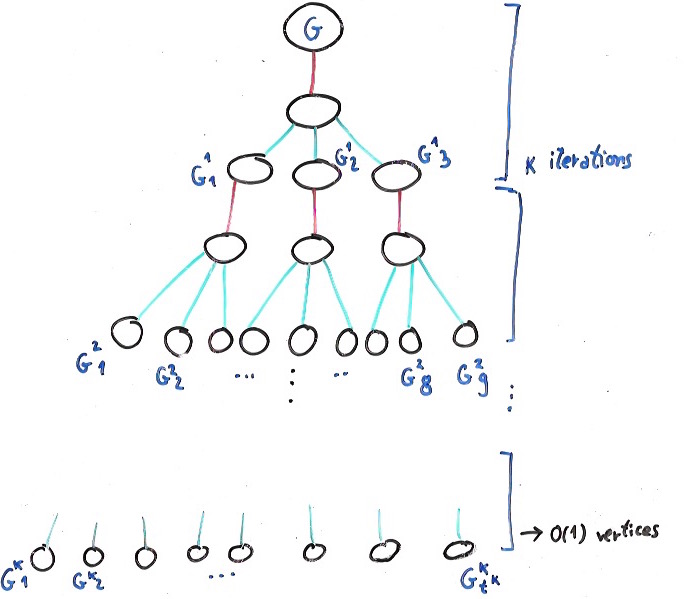
Figure 22: The recursion tree used for constructing an oblivious routing on \(G\), with \(t = 3\). Green lines correspond to applying edge sparsification, and red lines correspond to applying vertex elimination.
11.5.6.3 Proof of the vertex elimination theorem
In this section, we present the proof of the vertex elimination theorem. A key ingredient, also used in the proof of the edge sparsification theorem, is the notion of embedding.
Given two capacitated graphs \(G = (V, E, \mu)\) and \(G' = \left(V, E', \mu'\right)\) with the same vertex set and with edge-vertex incidence matrices \(B\) and \(B'\), an embedding from \(G\) to \(G'\) is a matrix \(M \in \mathbb{R}^{E' \times E}\) such that \(B'^\intercal M = B^\intercal\). If we let \(f \in \mathbb{R}^E\), then we have \(Mf \in \mathbb{R}^{E'}\) and \(B'^\intercal (M f) = B^\intercal f\). Thus, an embedding \(M\) from \(G\) to \(G'\) allows mapping a flow \(f\) on \(G\) to a flow \(f' = Mf\) on \(G'\) satisfying the same vertex demands.
Recall that the vertex elimination theorem and the edge sparsification theorem require the ability to efficiently construct an oblivious routing with low congestion for a graph \(G\) by using oblivious routings for the simpler graphs obtained from \(G\). Next, we show that embeddings allow us to do that.
The congestion of an embedding \(M\) is defined as the maximum factor by which the congestion increases when we use \(M\) to construct a flow in \(G'\) using a flow in \(G\). More precisely, we have $$\textrm{conge}(M) = \max_{x \in \mathbb{R}^E \setminus \{\vec{0}\} } \frac{\left\|U'^{-1}Mx\right\|_{\infty}}{\left\|U^{-1}x \right\|_{\infty}} \ ,\notag$$ where \(U\) and \(U'\) denote the edge capacities matrices of \(G\) and \(G'\) respectively. Making a change of variable \(x = Ux'\) yields $$\begin{aligned} \textrm{conge}(M) & = & \max_{x' \in \mathbb{R}^E \setminus \{\vec{0}\}} \frac{\left\|U'^{-1}MUx'\right\|_{\infty}}{\left\|x' \right\|_{\infty}} \\ & = & \left\|U'^{-1}MU\right\|_{\infty} \ . \end{aligned}\notag$$
The following lemma shows that, as long as two graphs \(G\) and \(G'\) can be embedded into each other with low congestion, it is easy to construct an oblivious routing on one of them using an oblivious routing on the other, without increasing the competitive ratio by much.
Let \(G = (V, E, \mu)\) and \(G' = \left(V, E', \mu'\right)\) be two capacitated graphs with the same vertex set. Let \(M\) (respectively, \(M'\)) be an embedding from \(G\) to \(G'\) (respectively, from \(G'\) to \(G\)). If \(A'\) is an oblivious routing on \(G'\), then \(A = M'A'\) is an oblivious routing on \(G\) with congestion $$\rho(A) \le \textrm{conge}(M)\textrm{conge}\left(M'\right)\rho\left(A'\right) \ .\label{lemm_emb}$$
Let \(G\) (respectively, \(G'\)) have edge capacities matrix \(U\) (respectively, \(U'\)) and edge-vertex incidence matrix \(B\) (respectively, \(B'\)).
First, note that \(A\) is indeed an oblivious routing on \(G\): for a vector of vertex demands \(\chi \in \mathbb{R}^V\), we have $$\begin{aligned} B^\intercal A\chi & = & B^\intercal\left(M'A'\right)\chi\\ & = & B^\intercal\underbrace{\left(M'\underbrace{\left(A'\chi\right)}_{\textrm{flow in }G' \textrm{ satisfying vertex demands } \chi}\right)}_{\textrm{flow in } G \textrm{ satisfying vertex demands } \chi} \\ & = & \chi \ . \end{aligned}\notag$$
To conclude, we bound the competitive ratio of \(A\). We have $$\begin{aligned} \rho(A) & = & \left\|U^{-1}AB^\intercal U\right\|_{\infty} \\ &= & \left\|U^{-1}M'A'B^\intercal U\right\|_{\infty}\\ &= &\left\|U^{-1}M'A'\left(B'^\intercal M\right)U\right\|_{\infty} \\ & = & \left\|U^{-1}M'U'U'^{-1}A'B'^\intercal U'U'^{-1}MU\right\|_{\infty} \\ & \le & \left\|U^{-1}M'U'\right\|_{\infty} \left\|U'^{-1} A'B'^\intercal U'\right\|_{\infty} \left\|U'^{-1}MU\right\|_{\infty} \\ & = & \textrm{conge}(M')\rho\left(A'\right)\textrm{conge}\left(M\right) \ . \end{aligned}\notag$$
11.5.6.3.1 From graphs to partial tree embedding graphs
In this section, we describe how to reduce obtaining a low-congestion oblivious routing on \(G\) to obtaining oblivious routings on \(t\) subgraphs \(H_1, \dots, H_t\) of \(G\) with fewer edges. These graphs will be partial tree embedding graphs.
Before giving the definition of a partial tree embedding graph, we need to introduce some notation related to spanning trees. Let \(T\) be a spanning tree of \(G\). Note that removing a subset \(F \subseteq T\) of the edges of the tree breaks it into multiple connected components. We say that the edges of \(G\) with endpoints in different components are cut by \(F\), and we denote the set of such edges by \(\partial_T(F)\). When \(F = \{e\}\) is a singleton, we abuse notation and write \(\partial_T(e)\) instead of \(\partial_T(\{e\})\), and say that the edges of \(\partial_T(e)\) are cut by \(e\).
We define the load on an edge \(e \in T\) of the spanning tree to be the sum of the capacities of all edges cut by \(e\), that is, $$\textrm{load}_T(e) = \sum_{e' \in \partial_T(e)} \mu_{e'} \ .\notag$$
We are now ready to define a partial tree embedding graph. Given a spanning tree \(T\) of \(G\) and a subset of the edges of the spanning tree \(F \subseteq T\), we define a capacitated graph \(H = H(G, T, F) = \left(V, E', \mu'\right)\) as follows:
- the vertex set is the same as the vertex set of \(G\);
- \(H\) contains the edges of the spanning tree and the edges cut by \(F\), that is, \(E' = T \cup \partial_T(F)\);
- the capacities of the edges of \(H\) are unchanged, except for the edges which are in the tree but not in \(F\), which have their capacity changed to their loads, that is, we define $$\mu'_e = \begin{cases} \textrm{load}_T(e) & \textrm{, if } e\in T\setminus F, \\ \mu_e & \textrm{, otherwise.} \end{cases}\notag$$
We call a graph \(H\) obtained in this way a partial tree embedding graph. Figure 23 illustrates this definition. Let us define embeddings between \(G\) and \(H\). We denote by \(M_H \in \mathbb{R}^{E' \times E}\) the embedding from \(G\) to \(H\) which routes edges not cut by \(F\) over the tree, and routes all other edges over themselves. We denote by \(M'_{H} \in \mathbb{R}^{E \times E'}\) the embedding from \(H\) to \(G\) which maps all edges of \(H\) to themselves.
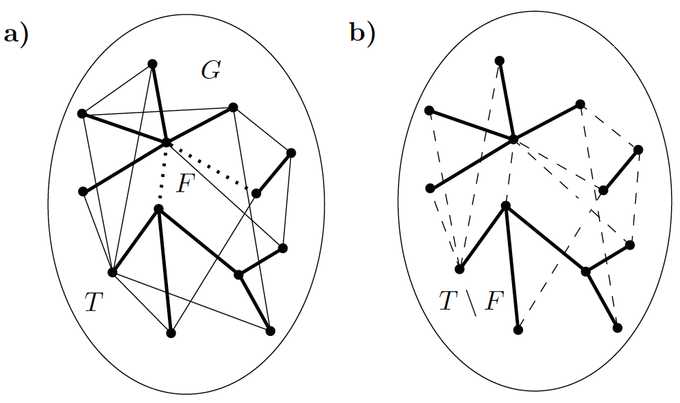
Figure 23: An example of a partial tree embedding, taken from Madry. In (a), we have the graph \(G\) (all edges), a spanning tree \(T\) (bold and dotted edges), and a subset \(F\) of the spanning tree (dotted edges). In (b), we have the partial tree embedding graph \(H(G, T, F)\). Note that the dotted edges in (b) form the set \(\partial_T(F)\).
The embedding \(M_H\) from \(G\) to \(H\) satisfies $$\textrm{conge}\left(M_H\right) \le 1 \ .\notag$$
Let \(f\) be a flow on \(G\), and let \(f' = M_Hf\) be the flow on \(H\) obtained by using the embedding \(M_H\).
Note that the capacity of each edge of \(H\) is greater than or equal to its capacity in \(G\). Thus, on the edges \(e \in E'\) such that \(f'_e \le f_e\), the congestion does not increase. It is thus sufficient to prove that the congestion with respect to the flow \(f'\) of edges on which we have an increase of flow, that is, \(f'_e > f_e\), is at most the congestion of the original flow \(f\).
Recall that \(M_H\) only reroutes the flow along the edges of \(G\) not cut by \(F\), using tree paths. Thus, the rerouting process only increases the flow on edges in \(T \setminus F\). Let \(e \in T \setminus F\) be such an edge, and note that its congestion with respect to the flow \(f'\) is $$\begin{aligned} \frac{f'_e}{\mu'_e} & = & \frac{\sum_{e' \in \partial_T(e)} f_{e'}}{\textrm{load}_T(e)} \\ & = & \frac{\sum_{e' \in \partial_T(e)} f_{e'}}{\sum_{e' \in \partial_T(e)} \mu_{e'}} \\ & \le & \frac{\sum_{e' \in \partial_T(e)} \left|f_{e'}\right|}{\sum_{e' \in \partial_T(e)} \mu_{e'}} \\ & \le & \max_{e'\in \partial_T(e)} \frac{\left|f_{e'}\right|}{\mu_{e'}} \\ & \le & \textrm{conge}(f) \ . \end{aligned}\notag$$
In order to be able to apply Lemma \ref{lemm_emb}, we would also need to embed \(H\) in \(G\) with low congestion, which is considerably harder. The following lemma shows that we can find a convex combination of partial tree embedding graphs such that the weighted sum of the congestions of the embeddings in the other direction is small.
(Madry) Given a capacitated graph \(G = (V, E, \mu)\) with capacity ratio \(S\) and \(t \in \mathbb{Z}_+^*\), we can find in \(\tilde{O}(tm)\) time a collection of partial tree embedding graphs \(H_1 = H\left(G, T_1, F_1\right), \dots, H_t = H\left(G, T_t, F_t\right)\) and coefficients \(\left(\lambda_i\right)_{i \in [t]}\) such that
- \(\left|F_i\right| = \tilde{O}\left(\frac{m\log{S}}{t}\right)\) for all \(i \in [t]\);
- \(\lambda_i \ge 0\) for all \(i \in [t]\);
- \(\sum_{i \in [t]} \lambda_i= 1\); and
- $$\sum_{i \in [t]} \lambda_i \textrm{conge}\left(M'_{H_i}\right) = \tilde{O}(1)\label{lemm_madry}$$.
Now that we have low congestion embeddings in both directions, we can use Lemma \ref{lemm_emb} to show that we can use low congestion oblivious routings on the graphs \(\left\{H_{i}\right\}_{i \in [t]}\) to obtain an oblivious routing with low congestion on \(G\).
Let \(A_i\) be an oblivious routing on \(H_i\), for each \(i \in [t]\). Then \(A = \sum_{i \in [t]}\lambda_i M'_{H_i}A_i\) is an oblivious routing on \(G\) with \(\rho(A) = \tilde{O}\left(\max_{i \in [t]}\rho(A_i)\right)\) and \(\mathcal{T}(A) = O\left(\sum_{i \in [t]} \mathcal{T}\left(A_i\right)\right)\label{lemm_t1}\).
We prove only the bound on the competitive ratio of \(A\). Let \(U_{H_i}\) denote the capacity matrix of \(H_i\), for all \(i \in [t]\). We have $$\begin{aligned} \rho(A) & = & \left\|U^{-1}AB^\intercal U\right\|_{\infty} \\ & = & \left\| U^{-1}\left(\sum_{i \in [t]} \lambda_i M'_{H_i}A_i\right)B^\intercal U\right\|_{\infty} \\ & \le & \sum_{i \in [t]} \lambda_i \left\| U^{-1} M'_{H_i}A_iB^\intercal U\right\|_{\infty} \\ & = & \sum_{i \in [t]} \lambda_i \left\| U^{-1} M'_{H_i}A_iB_{H_i}^\intercal M_{H_i}U\right\|_{\infty} \\ & = & \sum_{i \in [t]} \lambda_i \left\| U^{-1} M'_{H_i}U_{H_i}U_{H_i}^{-1}A_iB_{H_i}^\intercal U_{H_i}U_{H_i}^{-1}M_{H_i}U\right\|_{\infty} \\ & \le & \sum_{i \in [t]} \lambda_i \left\| U^{-1} M'_{H_i}U_{H_i}\right\|_{\infty} \left\|U_{H_i}^{-1}A_iB_{H_i}^\intercal U_{H_i}\right\|_{\infty} \left\|U_{H_i}^{-1}M_{H_i}U\right\|_{\infty} \\ & = & \sum_{i \in [t]} \lambda_i \textrm{conge}\left(M'_{H_i}\right) \rho\left(A_i\right) \underbrace{\textrm{conge}\left(M_{H_i}\right)}_{\le 1} \\ & \le & \max_{i \in [t]} \rho\left(A_i\right) \underbrace{\sum_{i \in [t]} \lambda_i \textrm{conge}\left(M'_{H_i}\right)}_{= \tilde{O}(1)} \\ & = & \tilde{O}\left(\max_{i \in [t]} \rho\left(A_i\right)\right) \ . \end{aligned}\notag$$
11.5.6.3.2 From partial tree embedding graphs to almost \(j\)-trees
In this section, we show that finding a low-congestion oblivious routing on a partial tree embedding graph reduces to finding an oblivious routing on an almost \(j\)-tree.
A graph \(G = \left(V, E\right)\) is an almost \(j\)-tree if it has a spanning tree \(T \subseteq E\) such that the edges of \(E \setminus T\) span at most \(j\) vertices. In other words, it is the union of a tree and a subgraph on at most \(j\) vertices. Figure 24 illustrates this definition.
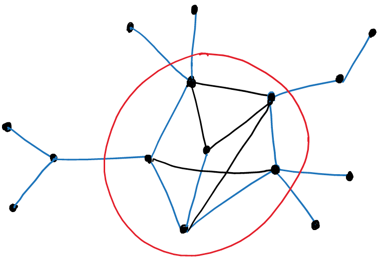
Figure 24: An almost \(j\)-tree for \(j = 6\). The blue edges form the spanning tree \(T\). The set of vertices inside the red circle form the core of \(G\), and the vertices outside it are called peripheral vertices.
Given a capacitated graph \(G = (V, E, \mu)\) and a partial tree embedding graph \(H = H(G, T, F)\), we can construct in \(\tilde{O}(m)\) time an almost \(2|F|\)-tree \(G' = \left(V, E', \mu'\right)\) and an embedding \(M'\) from \(G'\) to \(H\) such that
- \(\left|E'\right| \le m\);
- \(H\) is embeddable into \(G'\) with congestion \(2\);
- \(\textrm{conge}\left(M'\right) \le 2\); and
- $$\mathcal{T}\left(M'\right) = \tilde{O}(m)\label{lemm_partial}$$.
We describe how to construct the almost \(2|F|\)-tree \(G'\) and the embeddings from \(H\) to \(G'\) and vice-versa, but we do not prove that they have the required properties.
For an edge \(e = (u, v) \in E \setminus T\), consider the \(u\)-\(v\) path along the tree, and let \(v^1(e)\) be the first vertex that is incident to an edge of \(F\), and \(v^2(e)\) be the last one. For \(e \in T\), we set \(v^1(e) = u\) and \(v^2(e) = v\).
We define \(G' = \left(V, E', \mu'\right)\) as follows: the edge set is $$E' = \left\{\left(v^1(e),v^2(e)\right) : e \in E\right\} \ ,\notag$$ and the edge capacity of each edge \(e' \in E'\) is $$\mu'_{e'} = \sum_{\substack{e \in E \\ \left(v^1(e),v^2(e)\right) = e'}} \mu_e \ .\notag$$ Note that \(G'\) is an almost \(2|F|\)-tree, because by construction its edge set is composed by the spanning tree \(T\) and edges whose both endpoints are incident to edges of \(F\).
To embed \(H\) in \(G'\), we reroute the flow along each edge \(e = (u, v)\) of \(H\) as follows: we follow the \(u\)-\(v^1(e)\) tree path, then we take the edge \(\left(v^1(e),v^2(e)\right)\), then we follow the \(v^2(e)\)-\(v\) path. In other words, we shortcut the \(u\)-\(v\) tree path by using the edge \(\left(v^1(e), v^2(e)\right)\).
We can embed \(G'\) in \(H\) using a symmetric approach. Consider an edge \(e'\) of \(G'\), and let \(e = (u, v)\) be an edge of \(H\) such that \(\left(v^1(e), v^2(e)\right) = e'\). Then we could reroute the flow along edge \(e'\) by using the \(v^1(e)\)-\(u\) tree path, then the edge \(e\), then the \(v\)-\(v^2(e)\) tree path. Note that there might be multiple choices for the edge \(e\). We distribute the flow along \(e'\) among the different candidate paths, in such a way that the flow rerouted through the candidate path corresponding to edge \(e\) is proportional to its capacity \(\mu_e\).
11.5.6.3.3 From almost \(j\)-trees to fewer vertices
In this section, we show how to reduce finding a low-congestion oblivious routing in an almost \(j\)-tree \(G = (V, E, \mu)\) to finding a low-congestion oblivious routing in a graph with \(O(j)\) vertices.
To do that, we will show that vertices with degree \(1\) and \(2\) are easy to handle. After getting rid of those vertices, we get an almost \(j\)-tree in which all vertices have degree at least \(3\), and we show that such a graph has \(O(j)\) vertices.
We start by proving the last part.
If \(G = (V, E)\) is an almost \(j\)-tree with no degree \(1\) or degree \(2\) vertices, then $$|V| \le 3j - 2 \ .\notag$$
Let \(J \subseteq V\) be the core of \(G\), with \(|J| \le j\). Note that the graph obtained from \(G\) by removing the edges with both endpoints in \(J\) is a forest. Thus we have $$\begin{aligned} \label{ineq1} \sum_{v \in V \setminus J} \textrm{deg}(v) & \le & 2(|V\setminus J| -1) \notag\\ & \le & 2(|V| - 1) \ . \end{aligned}$$
On the other hand, since every vertex of \(G\) has degree at least \(3\), we have $$\begin{aligned} \label{ineq2} \sum_{v \in V \setminus J} \textrm{deg}(v) & \ge & 3|V \setminus J| \notag\\ & \ge & 3(|V| - j) \ . \end{aligned}$$
Inequalities \ref{ineq1} and \ref{ineq2} imply that $$3(|V| - j) \le 2(|V| - 1) \ ,\notag$$ and rearranging yields the result.
The following lemma shows that if we remove a degree \(1\) vertex, we can use an oblivious routing in the new graph to obtain an oblivious routing in the original graph, without changing the competitive ratio.
Let \(G = (V, E, \mu)\) be a capacitated graph, and let \(u \in V\) be a vertex incident to a unique edge \((u, v) \in E\). Let \(G = (V', E', \mu')\) be the graph that remains from removing the vertex \(u\) and the edge \((u, v)\). Given an oblivious routing \(A'\) in \(G'\), we can construct in \(O(1)\) time an oblivious routing \(A\) in \(G\) such that $$\rho(A) = \rho(A')\notag$$ and $$\mathcal{T}(A) = \mathcal{T\left(A'\right)} + O(1) \ .\label{lemm_leaf}$$
The key observation is the following:
(\(\star\)) Let \(\chi \in \mathbb{R}^V\) be a vector of vertex demands on \(G\). Then, for every flow \(f \in \mathbb{R}^E\) on \(G\) satisfying those vertex demands, since the edge \((u, v)\) is the only one that can be used to satisfy the demand of vertex \(u\), we must have \(f_u = \chi_u\).
Suppose we are given a vector of vertex demands \(\chi \in \mathbb{R}^V\) for graph \(G\). We can find a flow \(f \in \mathbb{R}^E\) in \(G\) satisfying those demands as follows: we start by setting \(f_{(u,v)} = \chi_u\) to satisfy the demand of vertex \(u\). Then we create a new vector of vertex demands \(\chi' \in \mathbb{R}^{V'}\) for graph \(G'\), by setting \(\chi'_v = \chi_v + \chi_u\) and \(\chi'_w = \chi_w\) for all other vertices \(w \in V' \setminus \{v\}\). Then, we use the oblivious routing \(A'\) on \(G'\) to obtain a flow \(f' = A'\chi'\) on \(G'\) satisfying vertex demands \(\chi'\). Now, we use that flow to complete our flow \(f\) on \(G\): we set \(f_{e} = f'_{e}\) for all edges \(e \in E \setminus \{(u, v)\}\). It is easy to see that the mapping \(A : \chi \mapsto f\) from vertex demands to flows that we just described is a linear oblivious routing on \(G\), and that \(\mathcal{T}(A) = \mathcal{T}\left(A'\right) + O(1)\).
Next, we show that the competitive ratios of \(A\) and \(A'\) are equal. To see that \(\rho(A) \ge \rho(A')\), it suffices to note that, given any set of vectors of vertex demands \(D' = \left\{\chi'^i\right\}_i\) for graph \(G'\), we can easily obtain a set of vertex demands \(D = \left\{\chi^i\right\}_i\) for graph \(G\) that will lead to the same ratio between the congestion obtained using oblivious routing and the optimal congestion: we can let \(\chi^i \in \mathbb{R}^{V}\) be defined as follows: $$\chi^i_w = \begin{cases} 0 & \textrm{, if } w = u, \\ \chi'^i_w & \textrm{, otherwise.} \end{cases}\notag$$
Next, we prove that that \(\rho(A) \le \rho(A')\). For a vector of vertex demands \(\chi \in \mathbb{R}^V\) for graph \(G\), we define a vector of vertex demands \(\chi' \in \mathbb{R}^{V'}\) on graph \(G'\) as follows: $$\chi'_w = \begin{cases} \chi_u + \chi_v & \textrm{, if } w = v, \\ \chi_w & \textrm{, otherwise.} \end{cases}\notag$$ For a set of vectors of vertex demands \(D = \left\{\chi^i\right\}_{i \in [k]}\) on \(G\), let \(D' = \left\{ \chi'^i \right\}_{i \in [k]}\) be the corresponding set of vectors of vertex demands on \(G'\). Using observation (\(\star\)), we can see that for every set of vectors of vertex demands \(D\) on \(G\), if we let $$c_\chi = \frac{\sum_{i \in [k]} \left|\chi^i_u\right|}{\mu_{(u,v)}} \ ,\notag$$ then we have $$\textrm{OPT}\left(D\right) = \max\left\{c_{\chi}, \textrm{OPT}\left(D'\right)\right\} \ .\notag$$ Moreover, by construction of \(A\) and \(A'\), we have $$\textrm{conge}\left(\left\{A\chi^i\right\}_{i \in [k]}\right) = \max\left\{c_{\chi}, \textrm{conge}\left(\left\{A'\chi'^i\right\}_{i \in [k]}\right) \right\} \ .\notag$$
Thus, we have $$\begin{aligned} \label{eqh} \rho(A) & = & \max_{D} \frac{\textrm{conge}\left(\left\{A\chi^i\right\}_{i \in [k]}\right)}{\textrm{OPT}(D)} \notag \\ & = & \max_{D} \frac{\max\left\{c_{\chi}, \textrm{conge}\left(\left\{A'\chi'^i\right\}_{i \in [k]}\right) \right\} }{ \max\left\{c_{\chi}, \textrm{OPT}\left(D'\right)\right\} } \ . \end{aligned}$$
We claim that for every \(D\), we have $$\label{eqg} \frac{\max\left\{c_{\chi}, \textrm{conge}\left(\left\{A'\chi'^i\right\}_{i \in [k]}\right) \right\} }{ \max\left\{c_{\chi}, \textrm{OPT}\left(D'\right)\right\} } \le \frac{ \textrm{conge}\left(\left\{A'\chi'^i\right\}_{i \in [k]}\right) }{ \textrm{OPT}\left(D'\right) } \ .$$
Now, to prove \ref{eqg}, we have three cases:
- if $$c_\chi \le \textrm{OPT}\left(D'\right) \ ,\notag$$ then we have $$\frac{\max\left\{c_{\chi}, \textrm{conge}\left(\left\{A'\chi'^i\right\}_{i \in [k]}\right) \right\} }{ \max\left\{c_{\chi}, \textrm{OPT}\left(D'\right)\right\} } = \frac{ \textrm{conge}\left(\left\{A'\chi'^i\right\}_{i \in [k]}\right) }{ \textrm{OPT}\left(D'\right) } \ ;\notag$$
- if $$\textrm{OPT}\left(D'\right) < c_\chi \le \textrm{conge}\left(\left\{A'\chi'^i\right\}_{i \in [k]}\right) \ ,\notag$$ then we have $$\begin{aligned} \frac{\max\left\{c_{\chi}, \textrm{conge}\left(\left\{A'\chi'^i\right\}_{i \in [k]}\right) \right\} }{ \max\left\{c_{\chi}, \textrm{OPT}\left(D'\right)\right\} } & = & \frac{ \textrm{conge}\left(\left\{A'\chi'^i\right\}_{i \in [k]}\right) }{ c_{\chi} } \\ & \le & \frac{ \textrm{conge}\left(\left\{A'\chi'^i\right\}_{i \in [k]}\right) }{ \textrm{OPT}\left(D'\right) }\ ; \end{aligned}\notag$$
- if $$\textrm{conge}\left(\left\{A'\chi'^i\right\}_{i \in [k]}\right) < c_\chi \ ,\notag$$ then we have $$\begin{aligned} \frac{\max\left\{c_{\chi}, \textrm{conge}\left(\left\{A'\chi'^i\right\}_{i \in [k]}\right) \right\} }{ \max\left\{c_{\chi}, \textrm{OPT}\left(D'\right)\right\} } & = & \frac{c_\chi}{c_{\chi}} \\ & = & 1 \\ & \le & \frac{ \textrm{conge}\left(\left\{A'\chi'^i\right\}_{i \in [k]}\right) }{ \textrm{OPT}\left(D'\right) } \ . \end{aligned}\notag$$
Now, note that \ref{eqh} and \ref{eqg} yield $$\begin{aligned} \rho(A) & \le & \max_{D} \frac{ \textrm{conge}\left(\left\{A'\chi'^i\right\}_{i \in [k]}\right) }{ \textrm{OPT}\left(D'\right) } \\ & \le & \rho\left(A'\right) \ , \end{aligned}$$ as desired.
The following lemma shows how to reduce constructing a low-congestion oblivious routing on an almost \(j\)-tree to constructing a low-congestion oblivious routing on an almost \(j\)-tree without vertices of degree \(1\) or \(2\), increasing the congestion by at most a factor of \(4\).
Given a capacitated almost \(j\)-tree \(G = (V, E, \mu)\), we can construct in \(O(m)\) time a capacitated graph \(G'\) such that, given an oblivious routing \(A'\) in \(G'\), we can construct in \(O(1)\) time an oblivious routing \(A\) in \(G\) such that $$\rho(A) \le 4\rho\left(A'\right)\notag$$ and $$\mathcal{T}(A) = O(\mathcal{T}\left(A'\right) + m) \ .\label{lemm_t3}$$
We sketch the construction presented in the paper. First, we repeatedly apply Lemma \ref{lemm_leaf} to remove degree \(1\) vertices. Let \(K\) be the resulting graph.
Next, consider each maximal path of the form \(\left(v_1, \dots, v_k\right)\), where \(k \ge 4\) and all internal vertices of the path have degree \(2\). For each such path, we let \(v_{j}v_{j+1}\) be the edge of smallest capacity. We remove the edge \(v_{j}v_{j+1}\) and add an edge \(v_1v_k\) with equal capacity. Note that this might introduce new vertices of degree \(1\). Let \(K'\) be the resulting graph. Repeatedly apply Lemma \ref{lemm_leaf} to remove degree \(1\) vertices, and let \(G'\) be the resulting graph. Then \(G'\) is an almost \(j\)-tree with no degree 1 or 2 vertices.
Note that \(K\) is embeddable in \(K'\) with congestion 2: we route every edge through itself, except the removed edges. If \(v_{j}v_{j + 1}\) is an edge which was removed from a path \(\left(v_1, \dots, v_k\right)\), then we reroute its flow through the path from \(v_j\) to \(v_1\), then the edge \(v_1v_k\), then the path from \(v_k\) to \(v_{j + 1}\).
One can also embed \(K\) in \(K'\) with congestion \(2\) in a symmetric manner. We route every edge through itself, except the newly added edges. If \(v_1v_k\) was added because of the path \(\left(v_1, \dots, v_k\right)\), then we reroute its flow through that path.
Note that the transformations from \(G\) to \(K\) and from \(K'\) to \(G'\) do not cause any loss in the competitive ratio, because of Lemma \ref{lemm_leaf}. Since \(K\) and \(K'\) can be embedded in each other with congestion 2, Lemma \ref{lemm_emb} implies that the transformation from \(K\) to \(K'\) yields a loss of at most a factor of \(4\).
Figures 25 – 28 illustrate the operations on a sample graph.
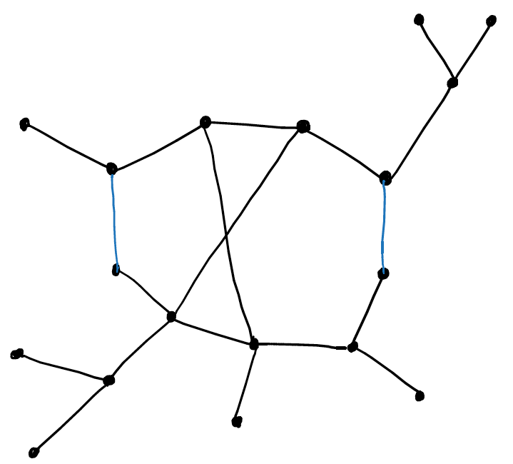
Figure 25: The starting graph \(G\). Black edges have capacity \(2\), while blue edges have capacity \(1\).
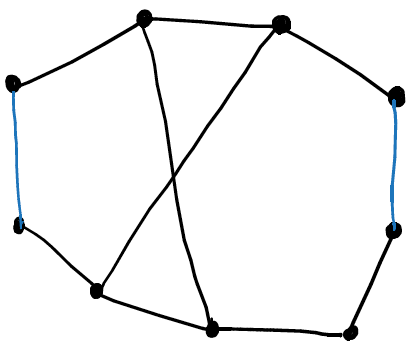
Figure 26: The graph \(K\) obtained by repeatedly removing degree 1 vertices.
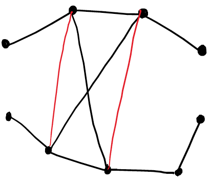
Figure 27: The graph \(K'\) obtained by removing the minimum capacity edge in each maximal path with internal vertices of degree 2 and adding an edge connecting its two extremities. The new (red) edges have capacity 1.
Figure 28: The graph \(G'\) obtained by repeatedly removing degree 1 vertices.
To conclude, we show how the vertex elimination lemma can be proved by combining Lemmas \ref{lemm_madry} – \ref{lemm_t3}. Using Lemma \ref{lemm_madry}, we construct \(t\) partial tree embedding graphs \(G_1, \dots, G_t\). Then we apply Lemma \ref{lemm_partial} to each of these graphs, obtaining \(t\) almost \(j\)-trees \(G'_1, \dots, G'_t\). Finally, applying Lemma \ref{lemm_t3} to each of these graphs, we obtain \(t\) graphs \(G''_1, \dots, G''_t\) satisfying the properties required by the vertex elimination lemma.