9. Continuous Probability Distributions
General Terminology and Notation
A continuous random variable is one for which the range (set
of possible values) is an interval (or a collection of intervals) on the real
number line. Continuous variables have to be treated a little differently than
discrete ones, the reason being that
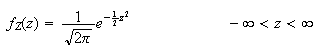
 has to be zero for each
 ,
in order to avoid mathematical contradiction. The distribution of a continuous
random variable is called a continuous probability
distribution. To illustrate, consider the simple spinning pointer in
Figure
spinner.
,
in order to avoid mathematical contradiction. The distribution of a continuous
random variable is called a continuous probability
distribution. To illustrate, consider the simple spinning pointer in
Figure
spinner.
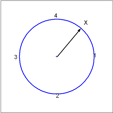
|
Spinner: a device for
generating a continuous random variable (in a zero-gravity, virtually
frictionless environment)
|
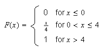
where all numbers in the
interval (0,4] are equally likely. The probability of the pointer stopping
precisely at the number
 must be zero, because if not the total probability for
 would be infinite, since the set
 is non-countable. Thus, for a continuous random variable the probability at
each point is 0. This means we can no longer use the probability function to
describe a distribution. Instead there are two other functions commonly used
to describe continuous distributions.
is non-countable. Thus, for a continuous random variable the probability at
each point is 0. This means we can no longer use the probability function to
describe a distribution. Instead there are two other functions commonly used
to describe continuous distributions.
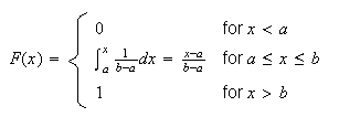
Cumulative Distribution Function:
For discrete random variables we defined the c.d.f.,
 .
This function still works for continuous random variables. For the spinner,
the probability the pointer stops between 0 and 1 is 1/4 if all values
.
This function still works for continuous random variables. For the spinner,
the probability the pointer stops between 0 and 1 is 1/4 if all values
 are equally ``likely"; between 0 and 2 the probability is 1/2, between 0 and 3
it is 3/4; and so on. In general,
are equally ``likely"; between 0 and 2 the probability is 1/2, between 0 and 3
it is 3/4; and so on. In general,
 for
for
 .
.
Also,
 for
for
 since there is no chance of the pointer stopping at a number
 ,
and
,
and
 for
for
 since the pointer is certain to stop at number below
 if
if
 .
.
Most properties of a c.d.f. are the same for continuous variables as for
discrete variables. These are:
1.
 and and
 |
2.
 is a non-decreasing function of
 |
3.
 . . |
Note that, as indicated before, for a continuous distribution, we have
 .
Also, since the probability is 0 at each point:
.
Also, since the probability is 0 at each point:
 (For a discrete random variable, each of these 4 probabilities could be
different.). For the continuous distributions in this chapter, we do not
worry about whether intervals are open, closed, or half-open since the
probability of these intervals is the
same.
(For a discrete random variable, each of these 4 probabilities could be
different.). For the continuous distributions in this chapter, we do not
worry about whether intervals are open, closed, or half-open since the
probability of these intervals is the
same.
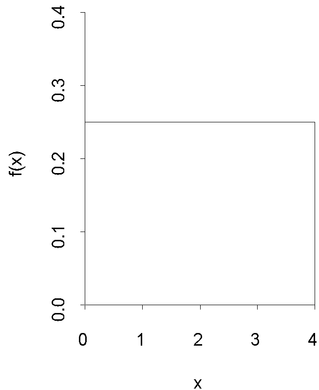
Probability Density Function (p.d.f.): While the c.d.f.
can be used to find probabilities, it does not give an intuitive picture of
which values of
 are more likely, and which are less likely. To develop such a picture suppose
that we take a short interval of
are more likely, and which are less likely. To develop such a picture suppose
that we take a short interval of
 -values,
![$[x,x+\Delta x]$](graphics/noteschap9__27.png) .
The probability
.
The probability
 lies in the interval is
 To compare the probabilities for two intervals, each of length
 ,
is easy. Now suppose we consider what happens as
,
is easy. Now suppose we consider what happens as
 becomes small, and we divide the probability by
 .
This leads to the following definition.
.
This leads to the following definition.
We will see that
 represents the relative likelihood of different
 -values.
To do this we first note some properties of a p.d.f. It is assumed that
-values.
To do this we first note some properties of a p.d.f. It is assumed that
 is a continuous function of
 at all points for which
 .
.
Properties of a probability density function
-
This
follows from the definition of
 .
.
-

(Since
 is non-decreasing).
-
This
is because
 .
.
-
 .
.
This is just property 1 with
 .
.
To see that
 represents the relative likelihood of different outcomes, we note that for
 small,
 Thus,
Thus,
 but
but
 is the approximate probability that
 is inside the interval
![$[x,x+\Delta x]$](graphics/noteschap9__57.png) .
A plot of the function
.
A plot of the function
 shows such values clearly and for this reason it is very common to plot the
p.d.f.'s of continuous random variables.
shows such values clearly and for this reason it is very common to plot the
p.d.f.'s of continuous random variables.
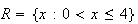
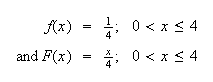
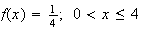
Example: Consider the spinner example, where
 Thus, the p.d.f. is
 ,
or
,
or
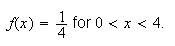 and outside this interval the p.d.f. is
 Figure
uniformpdf shows the probability density function
Figure
uniformpdf shows the probability density function
 ;
for obvious reasons this is called a "uniform" distribution.
;
for obvious reasons this is called a "uniform" distribution.
|
Uniform p.d.f.
|
Remark: Continuous probability distributions are, like
discrete distributions, mathematical models. Thus, the
distribution assumed for the spinner above is a model, though it seems likely
it would be a good model for many real spinners.
Remark: It may seem paradoxical that
 for a continuous r.v. and yet we record the outcomes
 in real "experiments" with continuous variables. The catch is that all
measurements have finite precision; they are in effect discrete. For example,
the height
in real "experiments" with continuous variables. The catch is that all
measurements have finite precision; they are in effect discrete. For example,
the height
 inches is within the range of the height
 of people in a population but we could never observe the outcome
 if we selected a person at random and measured their height.
To summarize, in measurements we are actually observing something like
 where
where
 may be very small, but not zero. The probability of this outcome is
not zero: it is (approximately)
may be very small, but not zero. The probability of this outcome is
not zero: it is (approximately)
 .
.
We now consider a more complicated mathematical example of a continuous random
variable Then we'll consider real problems that involve continuous variables.
Remember that it is always a good idea to sketch or plot the p.d.f.
 for a r.v.
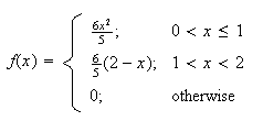
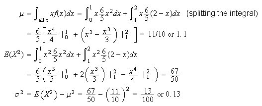
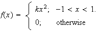
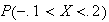
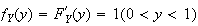
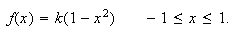
Example:
Let
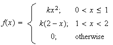 be a p.d.f.
Find
-

-

-
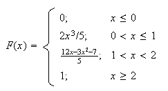
Solution:
-
Set
 to solve for
 .
When finding the area of a region bounded by different functions we split the
integral into pieces.
.
When finding the area of a region bounded by different functions we split the
integral into pieces.
(We normally wouldn't even write down the parts with
 )
)
-
Doing the easy pieces, which are often left out, first:
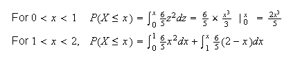
(see shaded area
below)
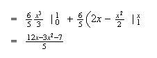
i.e.
As a rough check, since for a continuous distribution there is no probability
at any point,
 should have the same value as we approach each boundary point from above and
from below.
should have the same value as we approach each boundary point from above and
from below.
e.g.
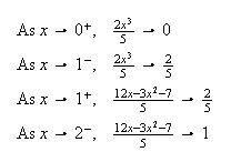
This quick check won't prove your answer is right, but will detect many
careless errors.
-
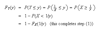
Defined Variables or Change of Variable:
When we know the
p.d.f. or c.d.f. for a continuous random variable
 we sometimes want to find the p.d.f. or c.d.f. for some other random variable
 which is a function of
 .
The procedure for doing this is summarized below. It is based on the fact that
the c.d.f.
.
The procedure for doing this is summarized below. It is based on the fact that
the c.d.f.
 for
for
 equals
 ,
and this can be rewritten in terms of
,
and this can be rewritten in terms of
 since
since
 is a function of
 .
Thus:
.
Thus:
-
Write the c.d.f. of
 as a function of
 .
.
-
Use
 to find
 .
Then if you want the p.d.f.
.
Then if you want the p.d.f.
 ,
you can differentiate the expression for
,
you can differentiate the expression for
 .
.
-
Find the range of values of
 .
.
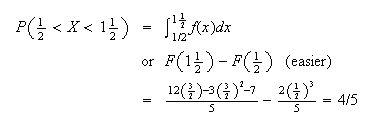
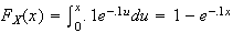
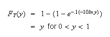
Example: In the earlier spinner example,
 Let
Let
 .
Find
.
Find
 .
.
Solution:
 For step (2), we can do either:
 (As
(As
 goes from 0 to 4,
 goes between
 and
and
 .)
.)
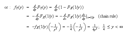 Generally if
 is known it is easier to substitute first, then differentiate. If
 is in the form of an integral that can't be solved, it is usually easier to
differentiate first, then substitute
is in the form of an integral that can't be solved, it is usually easier to
differentiate first, then substitute
 .
.
Extension of Expectation, Mean, and Variance to Continuous
Distributions
Definition
When
 is continuous, we still define
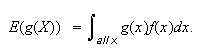
With this definition, all of the earlier properties of expectation and
variance still hold; for example with

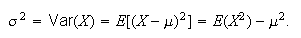
(This definition can be justified by writing
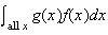 as a limit of a Riemann sum and recognizing the Riemann sum as being in the
form of an expectation for discrete random
variables.)
as a limit of a Riemann sum and recognizing the Riemann sum as being in the
form of an expectation for discrete random
variables.)
Example: In the spinner example with
Example: Let
 have p.d.f.
 Then
Then
Problems:
-
Let
 have p.d.f.
 Find
Find
-

-
the c.d.f.,

-
-
the mean and variance of
 .
.
-
let
 .
Derive the p.d.f. of
.
Derive the p.d.f. of
 .
.
-
A continuous distribution has c.d.f.
 for
for
 ,
where
,
where
 is a positive constant.
-
Evaluate
 .
.
-
Find the p.d.f.,
 .
.
-
What is the median of this distribution? (The median is the value of
 such that half the time we get a value below it and half the time above it.)
Continuous Uniform Distribution
Just as we did for discrete r.v.'s, we now consider some special types of
continuous probability distributions. These distributions arise in certain
settings, described below. This section considers what we call uniform
distributions.
Physical Setup:
Suppose
 takes values in some interval [a,b] (it doesn't actually matter whether
interval is open or closed) with all subintervals of a fixed length being
equally likely. Then
takes values in some interval [a,b] (it doesn't actually matter whether
interval is open or closed) with all subintervals of a fixed length being
equally likely. Then
 has a continuous uniform distribution. We write
 .
.
Illustrations:
-
In the spinner example
![$X \sim U (0,4]$](graphics/noteschap9__155.png) .
.
-
Computers can generate a random number
 which appears as though it is drawn from the distribution
 .
This is the starting point for many computer simulations of random processes;
an example is given below.
.
This is the starting point for many computer simulations of random processes;
an example is given below.
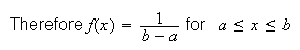
The probability density function and the cumulative distribution
function:
Since all points are equally likely (more precisely, intervals contained in
![$[a,b]$](graphics/noteschap9__158.png) of a given length, say 0.01, all have the same probability), the probability
density function must be a constant
of a given length, say 0.01, all have the same probability), the probability
density function must be a constant
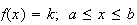 for some constant
 .
To make
.
To make
 ,
we require
,
we require
 .
.
Mean and
Variance: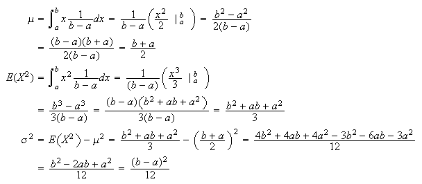
Example: Suppose
 has the continuous p.d.f.
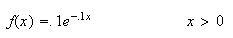 (This is called an exponential distribution and is discussed in the next
section. It is used in areas such as queueing theory and reliability.) We'll
show that the new random variable
(This is called an exponential distribution and is discussed in the next
section. It is used in areas such as queueing theory and reliability.) We'll
show that the new random variable
 has a uniform distribution,
 .
To see this, we follow the steps in Section
9.1:
.
To see this, we follow the steps in Section
9.1:
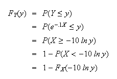
Since
 we get
(The range of
 is (0,1) since
 .)
Thus
.)
Thus
 and so
 .
.
Many computer software systems have ``random number generator" functions that
will simulate observations
 from a
 distribution. (These are more properly called pseudo-random number
generators because they are based on deterministic algorithms. In
addition they give observations
distribution. (These are more properly called pseudo-random number
generators because they are based on deterministic algorithms. In
addition they give observations
 that have finite precision so they cannot be exactly like
continuous
that have finite precision so they cannot be exactly like
continuous
 random variables. However, good generators give
 's
that appear indistinguishable in most ways from
's
that appear indistinguishable in most ways from
 r.v.'s.) Given such a generator, we can also simulate r.v.'s
 with the exponential distribution above by the following algorithm:
-
Generate
 using the computer random number generator.
-
Compute
 .
.
Then
 has the desired distribution. This is a particular case of a method described
in Section 9.4 for generating random variables from a general distribution. In
has the desired distribution. This is a particular case of a method described
in Section 9.4 for generating random variables from a general distribution. In
 software the command
 produces a vector consisting of
 independent
 values.
Problem:
-
If
 has c.d.f.
 ,
then
,
then
 has a uniform distribution on [0,1]. (Show this.) Suppose you want to simulate
observations from a distribution with
has a uniform distribution on [0,1]. (Show this.) Suppose you want to simulate
observations from a distribution with
 ,
by using the random number generator on a computer to generate
,
by using the random number generator on a computer to generate
 numbers. What value would
 take when you generated the random number .27125?
Exponential Distribution
The continuous random variable
 is said to have an exponential distribution if its p.d.f. is
of the form
is said to have an exponential distribution if its p.d.f. is
of the form
 where
where
 is a real parameter value. This distribution arises in various problems
involving the time until some event occurs. The following gives one such
setting.
is a real parameter value. This distribution arises in various problems
involving the time until some event occurs. The following gives one such
setting.
Physical Setup: In a Poisson process for events in time let
 be the length of time we wait for the first event occurrence. We'll show that
 has an exponential distribution. (Recall that the number of occurrences
in a fixed time has a Poisson distribution. The difference between the Poisson
and exponential distributions lies in what is being
measured.)
has an exponential distribution. (Recall that the number of occurrences
in a fixed time has a Poisson distribution. The difference between the Poisson
and exponential distributions lies in what is being
measured.)
Illustrations:
-
The length of time
 we wait with a Geiger counter until the emission of a radioactive particle is
recorded follows an exponential distribution.
we wait with a Geiger counter until the emission of a radioactive particle is
recorded follows an exponential distribution.
-
The length of time between phone calls to a fire station (assuming calls
follow a Poisson process) follows an exponential distribution.
Derivation of the probability density function and the c.d.f.
 |
= |
 (time to
 occurrence
 ) ) |
|
= |
 (time to
 occurrence
 )
) |
|
= |
 (no occurrences in the interval
 ) ) |
Check that you understand this last step. If the time to the first occurrence
 ,
there must be no occurrences in
,
there must be no occurrences in
 ,
and vice versa.
,
and vice versa.
We have now expressed
 in terms of the number of occurrences in a Poisson process by time
 .
But the number of occurrences has a Poisson distribution with mean
.
But the number of occurrences has a Poisson distribution with mean
 ,
where
,
where
 is the average rate of occurrence.
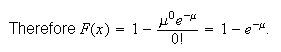 Since
Since
 for
for
 .
Thus
.
Thus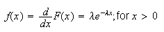 which is the formula we gave above.
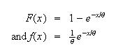
Alternate Form: It is common to use the parameter
 in the exponential distribution. (We'll see below that
 .)
This makes
.)
This makes
Exercise:
Suppose trees in a forest are distributed according to a Poisson process. Let
 be the distance from an arbitrary starting point to the nearest tree. The
average number of trees per square metre is
be the distance from an arbitrary starting point to the nearest tree. The
average number of trees per square metre is
 .
Derive
.
Derive
 the same way we derived the exponential p.d.f. You're now using the Poisson
distribution in 2 dimensions (area) rather than 1 dimension
(time).
the same way we derived the exponential p.d.f. You're now using the Poisson
distribution in 2 dimensions (area) rather than 1 dimension
(time).
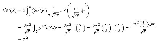
Mean and Variance:
Finding
 and
and
 directly involves integration by parts. An easier solution uses properties of
gamma functions, which extends the notion of factorials
beyond the integers to the positive real numbers.
directly involves integration by parts. An easier solution uses properties of
gamma functions, which extends the notion of factorials
beyond the integers to the positive real numbers.
Note that
 is 1 more than the power of
 in the integrand. e.g.
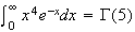 .
There are 3 properties of gamma functions which we'll use.
.
There are 3 properties of gamma functions which we'll use.
-
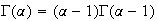 for
for

Proof:
Using integration by parts,
 and provided that

 Therefore
-
 if
if
 is a positive integer.
Proof: It is easy to show that
 Using property 1. repeatedly, we obtain
 etc.
etc.
Generally,.
 for integer

-

(This
can be proved using double
integration.)
Returning to the exponential distribution:
 Let
Let
 .
Then
.
Then
 and
and
Note: Read questions carefully. If you're given the average
rate of occurrence in a Poisson process, that is
 .
If you're given the average time you wait for an occurrence,
that is
.
If you're given the average time you wait for an occurrence,
that is
 .
.
To get
 ,
we first find
,
we first find
Example:
Suppose #7 buses arrive at a bus stop according to a Poisson process with an
average of 5 buses per hour. (i.e.
 /hr.
So
/hr.
So
 hr. or 12 min.) Find the probability (a) you have to wait longer than 15
minutes for a bus (b) you have to wait more than 15 minutes longer, having
already been waiting for 6 minutes.
hr. or 12 min.) Find the probability (a) you have to wait longer than 15
minutes for a bus (b) you have to wait more than 15 minutes longer, having
already been waiting for 6 minutes.
Solution:
-

=
-
If
 is the total waiting time, the question asks for the probability
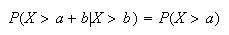
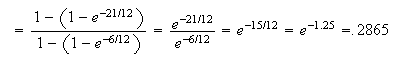 Does this surprise you? The fact that you're already waited 6 minutes doesn't
seem to matter. This illustrates the ``memoryless property'' of the
exponential distribution:
Does this surprise you? The fact that you're already waited 6 minutes doesn't
seem to matter. This illustrates the ``memoryless property'' of the
exponential distribution:
 Fortunately, buses don't follow a Poisson process so this example needn't
cause you to stop using the bus.
Fortunately, buses don't follow a Poisson process so this example needn't
cause you to stop using the bus.
Problems:
-
In a bank with on-line terminals, the time the system runs between disruptions
has an exponential distribution with mean
 hours. One quarter of the time the system shuts down within 8 hours of the
previous disruption. Find
hours. One quarter of the time the system shuts down within 8 hours of the
previous disruption. Find
 .
.
-
Flaws in painted sheets of metal occur over the surface according to the
conditions for a Poisson process, at an intensity of
 per
per
 .
Let
.
Let
 be the distance from an arbitrary starting point to the second closest flaw.
(Assume sheets are of infinite size!)
be the distance from an arbitrary starting point to the second closest flaw.
(Assume sheets are of infinite size!)
-
Find the p.d.f.,
 .
.
-
What is the average distance to the second closest flaw?
A Method for Computer Generation of Random Variables.
Most computer software has a built-in "pseudo-random number generator" that
will simulate observations
 from a
 distribution, or at least a reasonable approximation to this uniform
distribution. If we wish a random variable with a non-uniform distribution,
the standard approach is to take a suitable function of
distribution, or at least a reasonable approximation to this uniform
distribution. If we wish a random variable with a non-uniform distribution,
the standard approach is to take a suitable function of
 By far the simplest and most common method for generating non-uniform variates
is based on the inverse cumulative distribution function. For arbitrary c.d.f.
By far the simplest and most common method for generating non-uniform variates
is based on the inverse cumulative distribution function. For arbitrary c.d.f.
 ,
define
,
define
 min
min .
This is a real inverse (i.e.
.
This is a real inverse (i.e.
 )
in the case that the c.d.f. is continuous and strictly increasing, so for
example for a continuous distribution. However, in the more general case of a
possibly discontinuous non-decreasing c.d.f. (such as the c.d.f. of a discrete
distribution) the function continues to enjoy at least some of the properties
of an inverse.
)
in the case that the c.d.f. is continuous and strictly increasing, so for
example for a continuous distribution. However, in the more general case of a
possibly discontinuous non-decreasing c.d.f. (such as the c.d.f. of a discrete
distribution) the function continues to enjoy at least some of the properties
of an inverse.
 is useful for generating a random variables having c.d.f.
 from
from
 a uniform random variable on the interval
![$[0,1].$](graphics/noteschap9__281.png)
Proof:
The proof is a consequence of the fact that
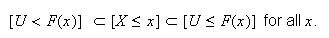 You can check this graphically be checking, for example, that if
![$[U<F(x)]$](graphics/noteschap9__288.png) then
then
![$[F^{-1}(U)\leq x]$](graphics/noteschap9__289.png) (this confirms the left hand
"
(this confirms the left hand
" Taking probabilities on all sides of this, and using the fact that
 ,
we discover that
,
we discover that
![$P[X\leq x]=F(x).$](graphics/noteschap9__292.png)
|
Inverting a c.d.f.
|
The relation
 implies that
 and for any point

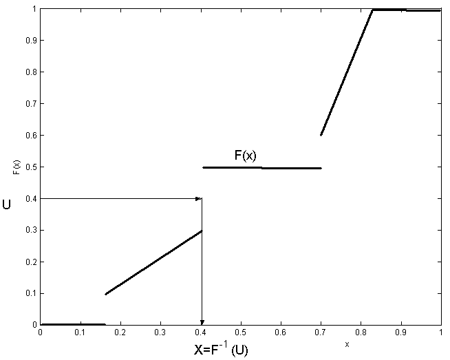
 For example, for the rather unusual looking piecewise linear cumulative
distribution function in Figure inversetransform, we
find the solution
For example, for the rather unusual looking piecewise linear cumulative
distribution function in Figure inversetransform, we
find the solution
 by drawing a horizontal line at
 until it strikes the graph of the c.d.f. (or where the graph would have been
if we had joined the ends at the jumps) and then
until it strikes the graph of the c.d.f. (or where the graph would have been
if we had joined the ends at the jumps) and then
 is the
 of this point. This is true in general,
 is the coordinate of the point where a horizontal line first strikes the graph
of the c.d.f. We provide one simple example of generating random variables by
this method, for the geometric distribution.
is the coordinate of the point where a horizontal line first strikes the graph
of the c.d.f. We provide one simple example of generating random variables by
this method, for the geometric distribution.
Example: A geometric random number generator
For the Geometric distribution, the cumulative distribution function is given
by
Then if
 is a uniform random number in the interval
![$[0,1],$](graphics/noteschap9__305.png) we seek an integer
we seek an integer
 such that
 (you should confirm that this is the value of
 at which the above horizontal line strikes the graph of the c.d.f) and solving
these inequalities gives
at which the above horizontal line strikes the graph of the c.d.f) and solving
these inequalities gives
 so we compute the value of
 and round down to the next lower integer.
Exercise: An exponential random number generator.
Show that the inverse transform method above results in the generator for the
exponential distribution
Normal Distribution
Physical Setup:
A random variable
 defined on
 has a normal distribution if it has probability density function of the form
 where
where
 and
and
 are parameters. It turns out (and is shown below) that
 and
Var
and
Var for this distribution; that is why its p.d.f. is written using the symbols
 and
and
 .
We write
.
We write
 to denote that
 has a normal distribution with mean
 and variance
 (standard deviation
 ).
).
The normal distribution is the most widely used distribution in probability
and statistics. Physical processes leading to the normal distribution exist
but are a little complicated to describe. (For example, it arises in physics
via statistical mechanics and maximum entropy arguments.) It is used for many
processes where
 represents a physical dimension of some kind, but also in many other settings.
We'll see other applications of it below. The shape of the p.d.f.
represents a physical dimension of some kind, but also in many other settings.
We'll see other applications of it below. The shape of the p.d.f.
 above is what is often termed a ``bell shape'' or ``bell curve'', symmetric
about
above is what is often termed a ``bell shape'' or ``bell curve'', symmetric
about
 as shown in Figure normpdf.(you should be able to
verify the shape without graphing the function)
as shown in Figure normpdf.(you should be able to
verify the shape without graphing the function)
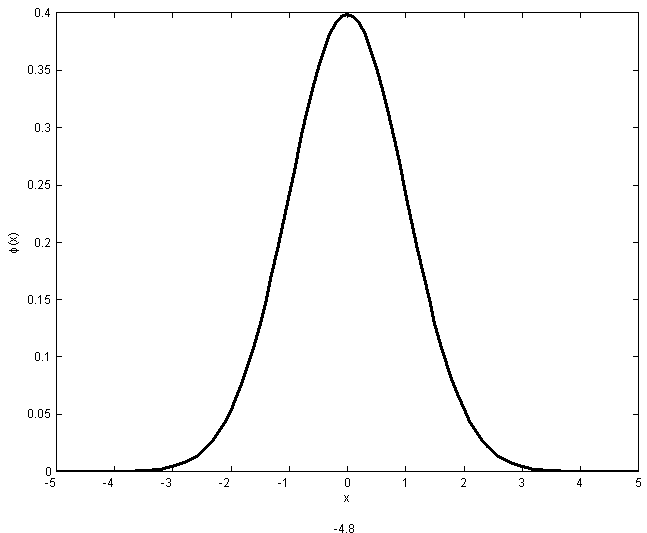
|
The standard normal
probability density function
|
Illustrations:
-
Heights or weights of males (or of females) in large populations tend to
follow normal distributions.
-
The logarithms of stock prices are often assumed to be normally distributed.
The cumulative distribution function: The c.d.f. of the
normal distribution
 is
is
 as shown in Figure normcdf. This integral cannot be
given a simple mathematical expression so numerical methods are used to
compute its value for given values of
as shown in Figure normcdf. This integral cannot be
given a simple mathematical expression so numerical methods are used to
compute its value for given values of
 and
and
 .
This function is included in many software packages and some calculators.
.
This function is included in many software packages and some calculators.
|
The standard normal c.d.f.
|
In the statistical packages
 and
and
 -Plus
we get
-Plus
we get
 above using the function
 .
.
Before computers, people produced tables of probabilities
 using mechanical calculators. Fortunately it is necessary to do this only for
a single normal distribution: the one with
using mechanical calculators. Fortunately it is necessary to do this only for
a single normal distribution: the one with
 and
and
 .
This is called the ``standard" normal distribution and
denoted
.
This is called the ``standard" normal distribution and
denoted
 .
.
Its easy to see that if
 then the "new" r.v.
 is distributed as
 .
(Just use the change of variables methods in Section 9.1.) We'll use this to
compute
.
(Just use the change of variables methods in Section 9.1.) We'll use this to
compute
 and probabilities for
 below, but first we show that
 integrates to 1 and that
 and
Var
and
Var .
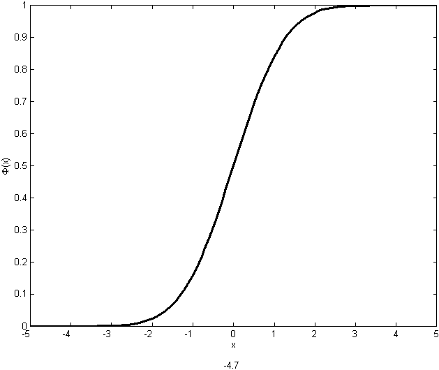
For the first result, note
that
.
For the first result, note
that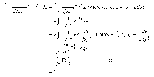
Mean, Variance, Moment generating function: Recall that an
odd function,
 ,
has the property that
,
has the property that
 .
If
.
If
 is an odd function then
 ,
provided the integral exists.
,
provided the integral exists.
Consider
Let
 .
Then
.
Then
where
 is an odd function so that
 .
But since
.
But since
 ,
this implies
,
this implies
 and so
 is the mean. To obtain the variance,
 We can obtain a gamma function by letting
 .
.
 Then
Then
 and so
 is the variance. We now find the moment generating function of the
 distribution. If
 has the
 distribution, then
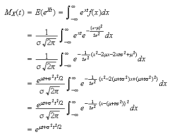 where the last step follows since
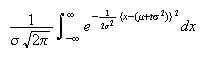 is just the integral of a
 probability density function and is therefore equal to one. This confirms the
values we already obtained for the mean and the variance of the normal
distribution
probability density function and is therefore equal to one. This confirms the
values we already obtained for the mean and the variance of the normal
distribution
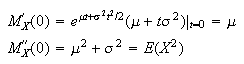 from which we obtain
Finding Normal Probabilities Via
 Tables As noted above,
 does not have an explicit closed form so numerical computation is needed. The
following result shows that if we can compute the c.d.f. for the standard
normal distribution
does not have an explicit closed form so numerical computation is needed. The
following result shows that if we can compute the c.d.f. for the standard
normal distribution
 ,
then we can compute it for any other normal distribution
,
then we can compute it for any other normal distribution
 as well.
Proof: The fact that
 has p.d.f.
 follows immediately by change of variables. Alternatively, we can just note
that
follows immediately by change of variables. Alternatively, we can just note
that
A table of probabilities
 is given on the last page of these notes. A space-saving feature is that only
the values for
is given on the last page of these notes. A space-saving feature is that only
the values for
 are shown; for negative values we use the fact that
 p.d.f. is symmetric about 0.
The following examples illustrate how to get probabilities for
 using the tables.
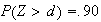
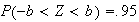
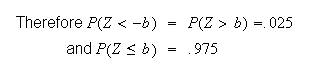
Examples: Find the following probabilities, where
 .
.
-

-

-

-

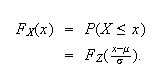
-
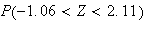
Solution:
-
Look up 2.11 in the table by going down the left column to 2.1 then across to
the heading .01. We find the number .9826. Then
 .
See Figure exercisenormal1.
.
See Figure exercisenormal1.
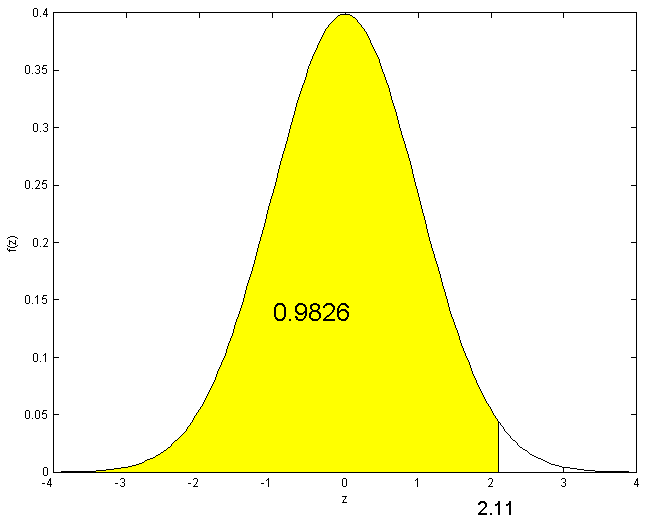
-

-

-
Now we have to use symmetry:
 See Figure exercisenormal2.
-


In addition to using the tables to find the probabilities for given numbers,
we sometimes are given the probabilities and asked to find the number. With
 or
or
 -Plus
software , the function qnorm
-Plus
software , the function qnorm
 gives the 100
 -th
percentile (where
-th
percentile (where
 .
We can also use tables to find desired values.
.
We can also use tables to find desired values.
Examples:
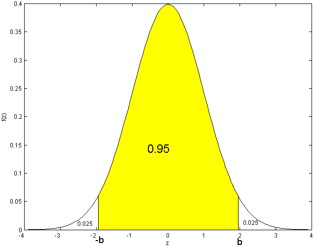
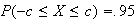
-
Find a number
 such that
-
Find a number
 such that
-
Find a number
 such that

Solutions:
-
We can look in the body of the table to get an entry close to .8500. This
occurs for
 between 1.03 and 1.04;
 gives the closest value to .85. For greater accuracy, the table at the bottom
of the last page is designed for finding numbers, given the probability.
Looking beside the entry .85 we find
gives the closest value to .85. For greater accuracy, the table at the bottom
of the last page is designed for finding numbers, given the probability.
Looking beside the entry .85 we find
 .
.
-
Since
 we have
 .
There is no entry for which
.
There is no entry for which
 so we again have to use symmetry, since
 will be negative.
The key to this solution lies in recognizing that
 will be negative. If you can picture the situation it will probably be easier
to handle the question than if you rely on algebraic
manipulations.
will be negative. If you can picture the situation it will probably be easier
to handle the question than if you rely on algebraic
manipulations.
Exercise: Will
 be positive or negative if
 ?
What if
?
What if
 ?
?
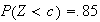
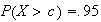
-
If
 we again use
symmetry.
we again use
symmetry.
The probability outside the interval
 must be .05, and this is evenly split between the area above
 and the area below
 .
.
Looking in the table,
 .
.
To find
 probabilities in general, we use the theorem given earlier, which implies that
if
probabilities in general, we use the theorem given earlier, which implies that
if
 then
then
 where
where
 .
.
Example: Let
 .
.
-
Find

-
Find a number
 such that
 .
.
Solution:
-
-
 Gaussian Distribution: The normal distribution is also known
as the Gaussian Note_1
distribution. The notation
Gaussian Distribution: The normal distribution is also known
as the Gaussian Note_1
distribution. The notation
 means that
 has Gaussian (normal) distribution with mean
 and standard deviation
 .
So, for example, if
.
So, for example, if
 then we could also write
 .
.
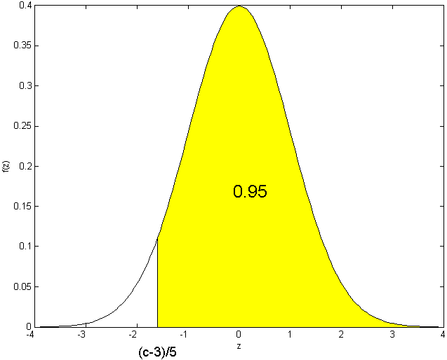
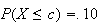
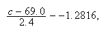
Example: The heights of adult males in Canada are close to
normally distributed, with a mean of 69.0 inches and a standard deviation of
2.4 inches. Find the 10th and 90th percentiles of the height distribution.
(Recall that the a-th percentile is such that a% of the population has height
less that this value.)
Solution: We are being told that if
 is the height of a randomly selected Canadian adult male, then
 ,
or equivalently
,
or equivalently
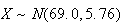 .
To find the 90th percentile
.
To find the 90th percentile
 ,
we
use
,
we
use From the table we see
 so we need
 which gives
 inches. Similarly, to find
 such that
 we find that
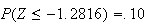 ,
so we need
,
so we need
 or
or
 inches, as the 10th percentile.
Linear Combinations of Independent Normal Random Variables
Linear combinations of normal r.v.'s are important in many applications. Since
we have not covered continuous multivariate distributions, we can only quote
the second and third of the following results without proof. The first result
follows easily from the change of variables method.
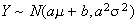
-
Let
 and
and
 ,
where
,
where
 and
and
 are constant real numbers. Then
-
Let
 and
and
 be independent, and let
 and
and
 be constants.
Then
 .
.
In
general if
 are independent and
 are constants,
then
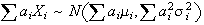 .
.
-
Let
 be independent
 random variables.
Then
 and
and
 .
.
Actually, the only new result here is that the distributions are normal. The
means and variances of linear combinations of r.v.'s were previously obtained
in section 8.3.
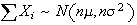
Example: Let
 and
and
 be independent. Find
 .
.
Solution: Whenever we have variables on both sides of the
inequality we should collect them on one side, leaving us with a linear
combination.
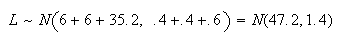
Example: Three cylindrical parts are joined end to end to
make up a shaft in a machine; 2 type A parts and 1 type B. The lengths of the
parts vary a little, and have the distributions:
 and
and
 .
The overall length of the assembled shaft must lie between 46.8 and 47.5 or
else the shaft has to be scrapped. Assume the lengths of different parts are
independent. What percent of assembled shafts have to be scrapped?
.
The overall length of the assembled shaft must lie between 46.8 and 47.5 or
else the shaft has to be scrapped. Assume the lengths of different parts are
independent. What percent of assembled shafts have to be scrapped?
Exercise: Why would it be wrong to represent the length of
the shaft as 2A + B? How would this length differ from the solution given
below?
Solution: Let
 ,
the length of the shaft, be
,
the length of the shaft, be
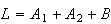 .
.
Then
 and so
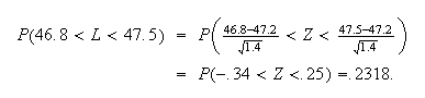
i.e. 23.18% are acceptable and 76.82% must be scrapped. Obviously we have to
find a way to reduce the variability in the lengths of the parts. This is a
common problem in manufacturing.
Exercise: How could we reduce the percent of shafts being
scrapped? (What if we reduced the variance of
 and
and
 parts each by 50%?)
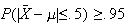
Example:
The heights of adult females in a large population is well represented by a
normal distribution with mean 64 in. and variance 6.2
in .
.
-
Find the proportion of females whose height is between 63 and 65 inches.
-
Suppose 10 women are randomly selected, and let
 be their average height ( i.e.
 ,
where
,
where
 are the heights of the 10 women). Find
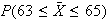 .
.
-
How large must
 be so that a random sample of
 women gives an average height
 so that
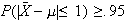 ?
?
Solution:
-
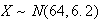 so for the height
 of a random
woman,
of a random
woman,
-
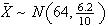 so
so
-
If
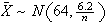 then
then
iff
 .
(This is because
.
(This is because
 .
So
.
So
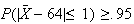 iff
iff
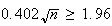 which is true if
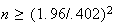 ,
or
,
or
 .
Thus we require
.
Thus we require
 since
since
 is an integer.
Remark: This shows that if we were to select a random sample
of
 persons, then their average height
 would be with 1 inch of the average height
 of the whole population of women. So if we did not know
 then we could estimate it to within
 inch (with probability .95) by taking this small a
sample.
inch (with probability .95) by taking this small a
sample.
Exercise: Find how large
 would have to be to make
 .
.
These ideas form the
basis of statistical sampling and estimation of unknown parameter values in
populations and processes. If
 and we know roughly what
 is, but don't know
 ,
then we can use the fact that
,
then we can use the fact that
 to find the probability that the mean
 from a sample of size
 will be within a given distance of
 .
.
Problems:
-
Let
 and
and
 be independent. Find the probability
-
-

-
 where
where
 is the sample mean of 25 independent observations on
 .
.
-
Let
 have a normal distribution. What percent of the time does
 lie within one standard deviation of the mean? Two standard deviations? Three
standard deviations?
lie within one standard deviation of the mean? Two standard deviations? Three
standard deviations?
-
Let
 .
An independent variable
.
An independent variable
 is also normally distributed with mean 7 and standard deviation 3. Find:
-
The probability
 differs from
 by more than 4.
-
The minimum number,
 ,
of independent observations needed on
,
of independent observations needed on
 so
that
so
that
 is the sample mean)
Use of the Normal Distribution in Approximations
The normal distribution can, under certain conditions, be used to approximate
probabilities for linear combinations of variables having a non-normal
distribution. This remarkable property follows from an amazing result called
the central limit theorem. There are actually several versions of the central
limit theorem. The version given below is one of the
simplest.
Central Limit Theorem (CLT):
The major reason that the normal distribution is so commonly used is that it
tends to approximate the distribution of sums of random variables. For
example, if we throw
 fair dice and
 is the sum of the outcomes, what is the distribution of
 The tables below provide the number of ways in which a given value can be
obtained. The corresponding probability is obtained by dividing by
The tables below provide the number of ways in which a given value can be
obtained. The corresponding probability is obtained by dividing by
 For example on the throw of
 dice the probable outcomes are 1,2,...,6 with probabilities all
 as indicated in the first panel of the histogram in Figure
clt.
as indicated in the first panel of the histogram in Figure
clt.
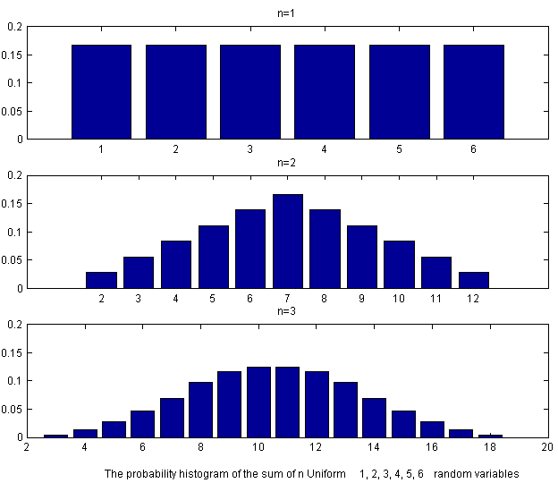
The probability histogram of
the sum of
 discrete uniform {1,2,3,4,5,6}Random variables
|
If we sum the values on two fair dice, the possible outcomes are the values
2,3,...,12 as shown in the following table and the probabilities are the
values below:
| Values |
2 |
3 |
4 |
5 |
6 |
7 |
8 |
9 |
10 |
11 |
12 |
Probabilities |
1 |
2 |
3 |
4 |
5 |
6 |
5 |
4 |
3 |
2 |
1 |
The probability histogram of these values is shown in the second panel.
Finally for the sum of the values on three independent dice, the values range
from 3 to 18 and have probabilities which, when multiplied by
 result in the values
to which we can fit three separate quadratic functions one in
the middle region and one in each of the two tails. The histogram of these
values shown in the third panel of Figure clt. and
already resembles a normal probability density function.In general, these
distributions show a simple pattern. For
 ,
the probability function is a constant (polynomial degree 0). For
,
the probability function is a constant (polynomial degree 0). For
 two linear functions spliced together. For
 ,
the histogram can be constructed from three quadratic pieces (polynomials of
degree
,
the histogram can be constructed from three quadratic pieces (polynomials of
degree
 These probability histograms rapidly approach the shape of the normal
probability density function, as is the case with the sum or the average of
independent random variables from most distributions. You can simulate the
throws of any number of dice and illustrate the behaviour of the sums on at
the url
http://www.math.csusb.edu/faculty/stanton/probstat/clt.html.
These probability histograms rapidly approach the shape of the normal
probability density function, as is the case with the sum or the average of
independent random variables from most distributions. You can simulate the
throws of any number of dice and illustrate the behaviour of the sums on at
the url
http://www.math.csusb.edu/faculty/stanton/probstat/clt.html.
Let
 be independent random variables all having the same distribution, with mean
 and variance
 .
Then as
.
Then as
 ,
,
 and
and
 This is actually a rough statement of the result since, as
 ,
both the
,
both the
 and
and
 distributions fail to exist. (The former because both
 and
and
 ,
the latter because
,
the latter because
 .)
A precise version of the results is:
.)
A precise version of the results is:
Although this is a theorem about limits, we will use it when
 is large, but finite, to approximate the distribution of
 or
or
 by a normal distribution, so the rough version of the theorem in
(cltsum) and (cltmean) is
adequate for our purposes.
by a normal distribution, so the rough version of the theorem in
(cltsum) and (cltmean) is
adequate for our purposes.
Notes:
-
This theorem works for essentially all distributions which
 could have. The only exception occurs when
 has a distribution whose mean or variance don't exist. There are such
distributions, but they are rare.
has a distribution whose mean or variance don't exist. There are such
distributions, but they are rare.
-
We will use the Central Limit Theorem to approximate the distribution of sums
 or averages
 .
The accuracy of the approximation depends on
.
The accuracy of the approximation depends on
 (bigger is better) and also on the actual distribution the
 's
come from. The approximation works better for small
's
come from. The approximation works better for small
 when
when
 's
p.d.f. is close to symmetric.
's
p.d.f. is close to symmetric.
-
If you look at the section on linear combinations of independent normal random
variables you will find two results which are very similar to the central
limit theorem. These are:
For
 independent and
 ,
,
 ,
and
,
and
 .
.
Thus, if the
 's
themselves have a normal distribution, then
's
themselves have a normal distribution, then
 and
and
 have exactly normal distributions for all values of
 .
If the
.
If the
 's
do not have a normal distribution themselves, then
's
do not have a normal distribution themselves, then
 and
and
 have approximately normal distributions when
 is large. From this distinction you should be able to guess that if the
 's
distribution is somewhat normal shaped the approximation will be good for
smaller values of
's
distribution is somewhat normal shaped the approximation will be good for
smaller values of
 than if the
 's
distribution is very non-normal in shape. (This is related to the second
remark in (2)).
's
distribution is very non-normal in shape. (This is related to the second
remark in (2)).
Example: Hamburger patties are packed 8 to a box, and each
box is supposed to have 1 Kg of meat in it. The weights of the patties vary a
little because they are mass produced, and the weight
 of a single patty is actually a random variable with mean
 kg and standard deviation
 kg. Find the probability a box has at least 1 kg of meat, assuming that the
weights of the 8 patties in any given box are
independent.
kg. Find the probability a box has at least 1 kg of meat, assuming that the
weights of the 8 patties in any given box are
independent.
Solution: Let
 be the weights of the 8 patties in a box, and
 be their total weight. By the Central Limit Theorem,
 is approximately
 ;
we'll assume this approximation is reasonable even though
;
we'll assume this approximation is reasonable even though
 is small. (This is likely ok because
 's
distribution is likely fairly close to normal itself.) Thus
's
distribution is likely fairly close to normal itself.) Thus
 and
and
 (We see that only about 95% of the boxes actually have 1 kg or more of
hamburger. What would you recommend be done to increase this probability to
95%?)
(We see that only about 95% of the boxes actually have 1 kg or more of
hamburger. What would you recommend be done to increase this probability to
95%?)
Example: Suppose fires reported to a fire station satisfy
the conditions for a Poisson process, with a mean of 1 fire every 4 hours.
Find the probability the
 fire of the year is reported on the
 day of the year.
Solution: Let
 be the time between the
 and
and
 fires
(
fires
( is the time to the
 fire). Then
 has an exponential distribution with
 hrs, or
 day. Since
 is the time until the 500th fire, we want to find
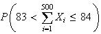 .
While the exponential distribution is not close to normal shaped, we are
summing a large number of independent exponential variables. Hence, by the
central limit theorem,
.
While the exponential distribution is not close to normal shaped, we are
summing a large number of independent exponential variables. Hence, by the
central limit theorem,
 has approximately a
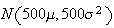 distribution, where
 and
and
 .
.
For exponential distributions,
 and
and
 so
so
Example: This example is frivolous but shows how the normal
distribution can approximate even sums of discrete r.v.'s. In an orchard,
suppose the number
 of worms in an apple has probability function:
 |
0 |
1 |
2 |
3 |
 |
.4 |
.3 |
.2 |
.1 |
Find the probability a basket with 250 apples in it has between 225 and 260
(inclusive) worms in it.
Solution:
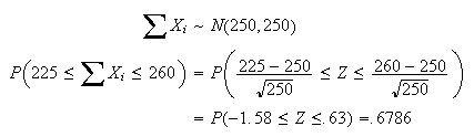
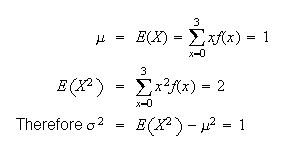 By the central limit theorem,
 has approximately a
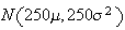 distribution, where
 is the number of worms in the
 apple.
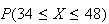
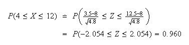
i.e.
While this approximation is adequate, we can improve its accuracy, as follows.
When
 has a discrete distribution, as it does here,
 will always remain discrete no matter how large
 gets. So the distribution of
 ,
while normal shaped, will never be precisely normal. Consider a probability
histogram of the distribution of
,
while normal shaped, will never be precisely normal. Consider a probability
histogram of the distribution of
 ,
as shown in Figure p167. (Only part of the histogram
is shown.)
,
as shown in Figure p167. (Only part of the histogram
is shown.)
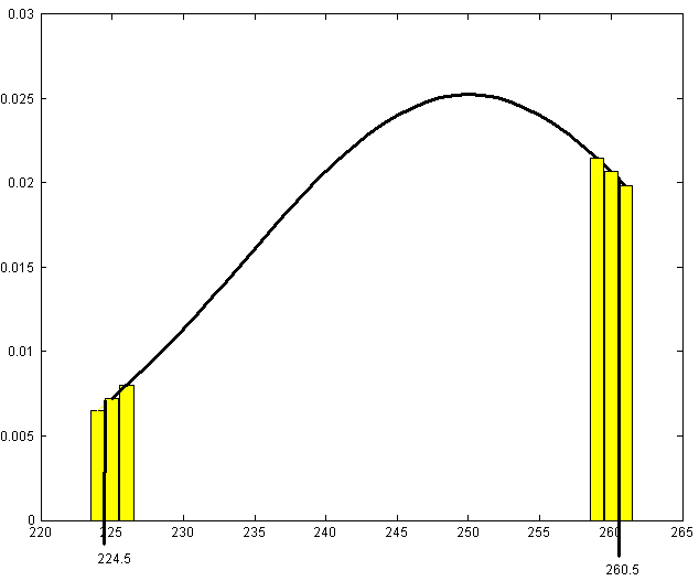
The area of each bar of this histogram is the probability at the
 value in the centre of the interval. The smooth curve is the p.d.f. for the
approximating normal distribution. Then
value in the centre of the interval. The smooth curve is the p.d.f. for the
approximating normal distribution. Then
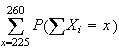 is the total area of all bars of the histogram for
 from 225 to 260. These bars actually span continuous
 values from 224.5 to 260.5. We could then get a more accurate approximation by
finding the area under the normal curve from 224.5 to 260.5.
values from 224.5 to 260.5. We could then get a more accurate approximation by
finding the area under the normal curve from 224.5 to 260.5.
i.e.

 Unless making this adjustment greatly complicates the solution, it is
preferable to make this "continuity
correction".
Unless making this adjustment greatly complicates the solution, it is
preferable to make this "continuity
correction".
Notes:
-
A continuity correction should not be applied when approximating a
continuous distribution by the normal distribution. Since it involves going
halfway to the next possible value of
 ,
there would be no adjustment to make if
,
there would be no adjustment to make if
 takes real values.
-
Rather than trying to guess or remember when to add .5 and when to subtract
.5, it is often helpful to sketch a histogram and shade the bars we wish to
include. It should then be obvious which value to
use.
Example: Normal approximation to the Poisson Distribution
Let
 be a random variable with a
Poisson
be a random variable with a
Poisson distribution and suppose
 is large. For the moment suppose that
 is an integer and recall that if we add
 independent Poisson random variables, each with parameter
 then the sum has the Poisson distribution with parameter
 In general, a Poisson random variable with large expected value can be written
as the sum of a large number of independent random variables, and so the
central limit theorem implies that it must be close to normally distributed.
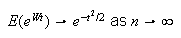
We can prove this using moment generating functions. In Section 7.5 we found
the moment generating function of a Poisson random variable
In general, a Poisson random variable with large expected value can be written
as the sum of a large number of independent random variables, and so the
central limit theorem implies that it must be close to normally distributed.
We can prove this using moment generating functions. In Section 7.5 we found
the moment generating function of a Poisson random variable

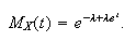 Then the standardized random variable is
 and this has moment generating function
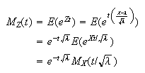 This is easier to work with if we take
logarithms,
This is easier to work with if we take
logarithms,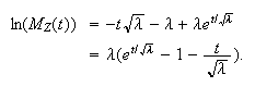 Now as

 and
and
 so
so
 Therefore the moment generating function of the standardized Poisson random
variable
Therefore the moment generating function of the standardized Poisson random
variable
 approaches
 the moment generating function of the standard normal and this implies that
the Poisson distribution approaches the normal as
the moment generating function of the standard normal and this implies that
the Poisson distribution approaches the normal as

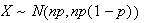
Normal approximation to the Binomial Distribution
It is well-known that the binomial distribution, at least for large values of
 resembles a bell-shaped or normal curve. The most common demonstration of this
is with a mechanical device common in science museums called a "Galton board"
or "Quincunx" Note_2 which drop
balls through a mesh of equally spaced pins (see Figure
balldrop and the applet at
resembles a bell-shaped or normal curve. The most common demonstration of this
is with a mechanical device common in science museums called a "Galton board"
or "Quincunx" Note_2 which drop
balls through a mesh of equally spaced pins (see Figure
balldrop and the applet at
http://javaboutique.internet.com/BallDrop/). Notice
that if balls either go to the right or left at each of the 8 levels of pins,
independently of the movement of the other balls, then
 number
of moves to right has a
number
of moves to right has a
 distribution. If the balls are dropped from location
 (on the
 axis)
then the ball eventually rests at location
axis)
then the ball eventually rests at location
 which is approximately normally distributed since
 is approximately normal.
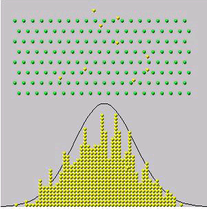
|
A "Galton Board" or
"Quincunx"
|
The following result is easily proved using the Central Limit
Theorem.![$\bigskip$]()
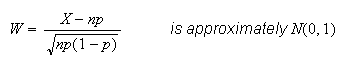
Proof: We use indicator variables
 where
where
 if the
 th
trial in the binomial process is an
"
th
trial in the binomial process is an
" " outcome
and 0 if it is an
"
" outcome
and 0 if it is an
" " outcome.
Then
" outcome.
Then
 and we can use the CLT. Since
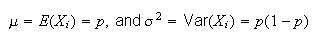 we have that as

 is
is
 ,
as stated. \framebox[0.10in]{}
,
as stated. \framebox[0.10in]{}
An alternative proof uses moment generating functions and is essentially a
proof of this particular case of the Central Limit Theorem. Recall that the
moment generating function of the binomial random variable
 is
is
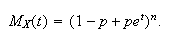 As we did with the standardized Poisson random variable, we can show with some
algebraic effort that the moment generating function of
As we did with the standardized Poisson random variable, we can show with some
algebraic effort that the moment generating function of

 proving that the standardized binomial random variable
 approaches the standard normal
distribution.
approaches the standard normal
distribution.![$\bigskip$]()
Remark: We can write the normal approximation either as
 or as
or as
 .
.![$\bigskip$]()
Remark: The continuity correction method can be used here.
The following numerical example illustrates the procedure.
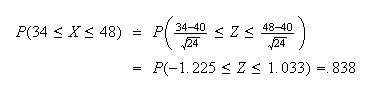
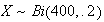
Example: If (i)
 ,
use the theorem to find the approximate probability
,
use the theorem to find the approximate probability
 and (ii) if
 find the approximate probability
 .
Compare the answer with the exact value in each
case.
.
Compare the answer with the exact value in each
case.![$\bigskip$]()
Solution (i) By the theorem above,
 approximately. Without the continuity correction,
 where
where
 .
Using the continuity correction method, we get
.
Using the continuity correction method, we get
 The exact probability is
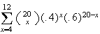 ,
which (using the
,
which (using the
 function
 )
is .963. As expected the continuity correction method gives a more accurate
approximation.
)
is .963. As expected the continuity correction method gives a more accurate
approximation.
(ii)
 approximately so without the continuity correction
 With the continuity correction
 The exact value,
 ,
equals .866 (to 3 decimals). The error of the normal approximation decreases
as
,
equals .866 (to 3 decimals). The error of the normal approximation decreases
as
 increases, but it is a good idea to use the CC when it is
convenient.
increases, but it is a good idea to use the CC when it is
convenient.
Example: Let
 be the proportion of Canadians who think Canada should adopt the US dollar.
-
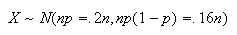
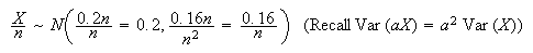
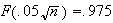
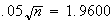
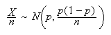
Suppose 400 Canadians are randomly chosen and asked their opinion. Let
 be the number who say yes. Find the probability that the proportion,
 ,
of people who say yes is within .02 of
,
of people who say yes is within .02 of
 ,
if
,
if
 is .20.
-
Find the number,
 ,
who must be surveyed so there is a 95% chance that
,
who must be surveyed so there is a 95% chance that
 lies within .02 of
 .
Again suppose
.
Again suppose
 is .20.
-
Repeat (b) when the value of
 is unknown.
Solution:
-
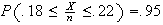
 .
Using the normal approximation we take
.
Using the normal approximation we take

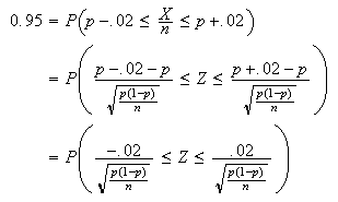
If
 lies within
 ,
then
,
then
 ,
so
,
so
 .
Thus, we find
.
Thus, we find
-
Since
 is unknown, it is difficult to apply a continuity correction, so we omit it in
this part. By the normal approximation,
is unknown, it is difficult to apply a continuity correction, so we omit it in
this part. By the normal approximation,
 Therefore,
 is the condition we need to satisfy. This
gives
is the condition we need to satisfy. This
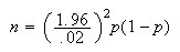
gives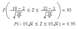 Therefore,
 and so
 giving
 In other words, we need to survey 1537 people to be at least 95% sure that
 lies within .02 either side of
 .
.
-
Now using the normal approximation to the binomial, approximately
 and
so
and
so
 We wish to find
 such that
 As is part
(b),
As is part
(b),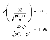 Solving for

 Unfortunately this does not give us an explicit expression for
 because we don't know
 .
The way out of this dilemma is to find the maximum value
.
The way out of this dilemma is to find the maximum value
 could take. If we choose
 this large, then we can be sure of having the required precision in our
estimate,
this large, then we can be sure of having the required precision in our
estimate,
 ,
for any
,
for any
 .
It's easy to see that
.
It's easy to see that
 is a maximum when
 .
Therefore we take
.
Therefore we take
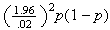
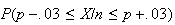
 i.e., if we survey 2401 people we can be 95% sure that
 lies within .02 of
 ,
regardless of the value of
,
regardless of the value of
 .
.
Remark: This method is used when poll results are reported
in the media: you often see or hear that "this poll is accurate to with 3
percent 19 times out of 20". This is saying that
 was big enough so that
 was 95%. (This requires
 of about 1067.)
Problems:
-
Tomato seeds germinate (sprout to produce a plant) independently of each
other, with probability 0.8 of each seed germinating. Give an expression for
the probability that at least 75 seeds out of 100 which are planted in soil
germinate. Evaluate this using a suitable approximation.
-
A metal parts manufacturer inspects each part produced. 60% are acceptable as
produced, 30% have to be repaired, and 10% are beyond repair and must be
scrapped. It costs the manufacturer $10 to repair a part, and $100 (in lost
labour and materials) to scrap a part. Find the approximate probability that
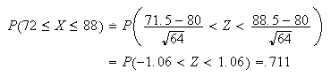
the total cost associated with inspecting 80 parts will exceed $1200.
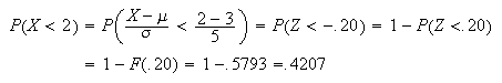
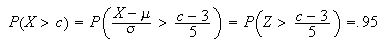
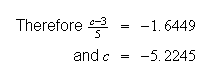
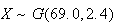
Problems on Chapter 9
-
The diameters
 of spherical particles produced by a machine are randomly distributed
according to a uniform distribution on [.6,1.0] (cm). Find the distribution of
of spherical particles produced by a machine are randomly distributed
according to a uniform distribution on [.6,1.0] (cm). Find the distribution of
 ,
the volume of a particle.
,
the volume of a particle.
-
A continuous random variable
 has p.d.f.
-
-
When people are asked to make up a random number between 0 and 1, it has been
found that the distribution of the numbers,
 ,
has p.d.f. close to
,
has p.d.f. close to
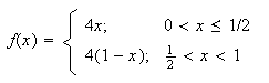 (rather than the
![$U[0,1]$](graphics/noteschap9__798.png) distribution which would be expected). Find the mean and variance of
distribution which would be expected). Find the mean and variance of
 .
.
-
For 100 ``random'' numbers from the above distribution find the probability
their sum lies between 49.0 and 50.5.
-
What would the answer to (b) be if the 100 numbers were truly
![$U[0,1]$](graphics/noteschap9__800.png) ?
?
-
Let
 have p.d.f.
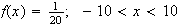 ,
and let
,
and let
 .
Find the p.d.f. of
.
Find the p.d.f. of
 .
.
-
A continuous random variable
 which takes values between 0 and 1 has probability density function
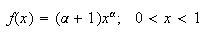
-
For what values of
 is this a p.d.f.? Explain.
-
Find
 and
and

-
Find the probability density function of
 .
.
-
The magnitudes of earthquakes in a region of North America can be modelled by
an exponential distribution with mean 2.5 (measured on the Richter scale).
-
If 3 earthquakes occur in a given month, what is the probability that none
exceed 5 on the Richter scale?
-
If an earthquake exceeds 4, what is the probability it also exceeds 5?
-
A certain type of light bulb has lifetimes that follow an exponential
distribution with mean 1000 hours. Find the median lifetime (that is, the
lifetime
 such that 50% of the light bulbs fail before
 ).
).
-
The examination scores obtained by a large group of students can be modelled
by a normal distribution with a mean of 65% and a standard deviation of 10%.
-
Find the percentage of students who obtain each of the following letter
grades:

-
Find the probability that the average score in a random group of 25 students
exceeds 70%.
-
Find the probability that the average scores of two distinct random groups of
25 students differ by more than 5%.
-
The number of litres
 that a filling machine in a water bottling plant deposits in a nominal two
litre bottle follows a normal distribution
that a filling machine in a water bottling plant deposits in a nominal two
litre bottle follows a normal distribution
 ,
where
,
where
 (litres) and
 is the setting on the machine.
-
If
 ,
what is the probability a bottle has less than 2 litres of water in it?
,
what is the probability a bottle has less than 2 litres of water in it?
-
What should
 be set at to make the probability a bottle has less than 2 litres be less than
 ?
?
-
A turbine shaft is made up of 4 different sections. The lengths of those
sections are independent and have normal distributions with
 and
and
 :
(8.10, .22), (7.25, .20),
:
(8.10, .22), (7.25, .20),
(9.75, .24), and (3.10, .20). What is the
probability an assembled shaft meets the specifications
 ?
?
-
Let
 and
and
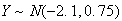 be independent.
Find:
-
-

-
a number
 such that
 .
.
-
The amount,
 ,
of wine in a bottle
,
of wine in a bottle
 (Note:
 means liters.)
-
The bottle is labelled as containing
 .
What is the probability a bottle contains less than
.
What is the probability a bottle contains less than
 ?
?
-
Casks are available which have a volume,
 ,
which is
,
which is
 .
What is the probability the contents of 20 randomly chosen bottles will fit
inside a randomly chosen cask?
.
What is the probability the contents of 20 randomly chosen bottles will fit
inside a randomly chosen cask?
-
In problem 8.18, calculate the probability of passing the exam, both with and
without guessing if (a) each
 = .45; (b) each
 .
.
What
is the best strategy for passing the course if (a)
 (b)
(b)
 ?
?
-
Suppose that the diameters in millimeters of the eggs laid by a large flock of
hens can be modelled by a normal distribution with a mean of 40 mm. and a
variance of 4
mm .
The wholesale selling price is 5 cents for an egg less than 37 mm in diameter,
6 cents for eggs between 37 and 42 mm, and 7 cents for eggs over 42 mm. What
is the average wholesale price per egg?
.
The wholesale selling price is 5 cents for an egg less than 37 mm in diameter,
6 cents for eggs between 37 and 42 mm, and 7 cents for eggs over 42 mm. What
is the average wholesale price per egg?
-
In a survey of
 voters from a given riding in Canada, the proportion
 who say they would vote Conservative is used to estimate
 ,
the probability a voter would vote P.C.
(
,
the probability a voter would vote P.C.
( is the number of Conservative supporters in the survey.) If Conservative
support is actually 16%, how large should
is the number of Conservative supporters in the survey.) If Conservative
support is actually 16%, how large should
 be so that with probability .95, the estimate will be in error at most .03?
-
When blood samples are tested for the presence of a disease, samples from 20
people are pooled and analysed together. If the analysis is negative, none of
the 20 people is infected. If the pooled sample is positive, at least one of
the 20 people is infected so they must each be tested separately; i.e., a
total of 21 tests is required. The probability a person has the disease is
.02.
-
Find the mean and variance of the number of tests required for each group of
20.
-
For 2000 people, tested in groups of 20, find the mean and variance of the
total number of tests. What assumption(s) has been made about the pooled
samples?
-
Find the approximate probability that more than 800 tests are required for the
2000 people.
-
Suppose 80% of people who buy a new car say they are satisfied with the car
when surveyed one year after purchase. Let
 be the number of people in a group of 60 randomly chosen new car buyers who
report satisfaction with their car. Let
be the number of people in a group of 60 randomly chosen new car buyers who
report satisfaction with their car. Let
 be the number of satisfied owners in a second (independent) survey of 62
randomly chosen new car buyers. Using a suitable approximation, find
be the number of satisfied owners in a second (independent) survey of 62
randomly chosen new car buyers. Using a suitable approximation, find
 .
A continuity correction is expected.
.
A continuity correction is expected.
-
Suppose that the unemployment rate in Canada is 7%.
-
Find the approximate probability that in a random sample of 10,000 persons in
the labour force, the number of unemployed will be between 675 and 725
inclusive.
-
How large a random sample would it be necessary to choose so that, with
probability
 ,
the proportion of unemployed persons in the sample is between 6.9% and 7.1%?
,
the proportion of unemployed persons in the sample is between 6.9% and 7.1%?
-
Gambling. Your chances of winning or losing money can be
calculated in many games of chance as described here.
Suppose each time you play a game (or place a bet) of $1 that the probability
you win (thus ending up with a profit of $1) is .49 and the probability you
lose (meaning your ``profit" is -$1) is .51
-
Let
 represent your profit after
 independent plays or bets. Give a normal approximation for the distribution of
 .
.
-
If
 ,
determine
,
determine
 .
(This is the probability you are ``ahead" after 20 plays.) Also find
.
(This is the probability you are ``ahead" after 20 plays.) Also find
 if
if
 and
and
 .
What do you conclude?
.
What do you conclude?
Note: For many casino games (roulette, blackjack) there are
bets for which your probability of winning is only a little less than .5.
However, as you play more and more times, the probability you lose (end up
``behind") approaches 1.
-
Suppose now you are the casino. If all players combined place
 $1 bets in an evening, let
 be your profit. Find the value
 with the property that
 .
Explain in words what this means.
.
Explain in words what this means.
-
Gambling: Crown and Anchor. Crown and Anchor is a game that
is sometimes played at charity casinos or just for fun. It can be played with
a ``wheel of fortune" or with 3 dice, in which each die has its 6 sides
labelled with a crown, an anchor, and the four card suits club, diamond, heart
and spade, respectively. You bet an amount (let's say $1) on one of the 6
symbols: let's suppose you bet on ``heart". The 3 dice are then rolled
simultaneously and you win
 if
if
 hearts turn up
(
hearts turn up
( ).
).
-
Let
 represent your profits from playing the game
 times. Give a normal approximation for the distribution of
 .
.
-
Find (approximately) the probability that
 if (i)
 ,
(ii)
,
(ii)
 .
.
-
Binary classification. Many situations require that we
``classify" a unit of some type as being one of two types, which for
convenience we will term Positive and Negative. For example, a diagnostic test
for a disease might be positive or negative; an email message may be spam or
not spam; a credit card transaction may be fraudulent or not. The problem is
that in many cases we cannot tell for certain whether a unit is Positive or
Negative, so when we have to decide which a unit is, we may make errors. The
following framework helps us to deal with these problems.
For a randomly selected unit from the population being considered, define the
indicator random variable
 Suppose that we cannot know for certain whether
 or
or
 for a given unit, but that we can get a measurement
 with the property that
 where
where
 .
We now decide to classify units as follows, based on their measurement
.
We now decide to classify units as follows, based on their measurement
 :
select some value
:
select some value
 between
 and
and
 ,
and then
,
and then
-
if
 ,
classify the unit as Positive
,
classify the unit as Positive
-
if
 ,
classify the unit as Negative
,
classify the unit as Negative
-
Suppose
 .
Find the probability that
.
Find the probability that
-
If a unit is really Positive, they are wrongly classified as Negative. (This
is called the ``false negative" probability.)
-
If a unit is really Negative, they are wrongly classified as Positive. (This
is called the ``false positive" probability.)
-
Repeat the calculations if
 as in (a), but
 .
Explain in plain English why the false negative and false positive
misclassification probabilities are smaller than in (a).
.
Explain in plain English why the false negative and false positive
misclassification probabilities are smaller than in (a).
-
Binary classification and spam detection. The approach in the
preceding question can be used for problems such as spam detection, which was
discussed earlier in Problems 4.17 and 4.18. Instead of using binary features
as in those problems, suppose that for a given email message we compute a
measure
 ,
designed so that
,
designed so that
 tends to be high for spam messages and low for regular (non-spam) messages.
(For example
tends to be high for spam messages and low for regular (non-spam) messages.
(For example
 can be a composite measure based on the presence or absence of certain words
in a message, as well as other features.) We will treat
can be a composite measure based on the presence or absence of certain words
in a message, as well as other features.) We will treat
 as a continuous random variable.
Suppose that for spam messages, the distribution of
 is approximately
 ,
and that for regular messages, it is approximately
,
and that for regular messages, it is approximately
 ,
where
,
where
 .
This is the same setup as for Problem 9.21. We will filter spam by picking a
value
.
This is the same setup as for Problem 9.21. We will filter spam by picking a
value
 ,
and then filtering any message for which
,
and then filtering any message for which
 .
The trick here is to decide what value of
.
The trick here is to decide what value of
 to use.
-
Random chords of a circle. Given a circle, find the
probability that a chord chosen at random be longer than the side of an
inscribed equilateral triangle. For example in Figure
bertrand, the line joining
 and
and
 satisfies the condition, the other lines do not.
|
Bertrand's Paradox
|
This is called Bertrand's
paradox (see the Java applet at http://www.cut-the-knot.org/bertrand.shtml)
and there various possible solutions, depending on exactly how you interpret
the phrase "a chord chosen at random". For example, since the only important
thing is the position of the second point relative to the first one, we can
fix the point
 and consider only the chords that emanate from this point. Then it becomes
clear that 1/3 of the outcomes (those with angle with the tangent at that
point between 60 and 120 degrees) will result in a chord longer than the side
of an equilateral triangle. But a chord is fully determined by its midpoint.
Chords whose length exceeds the side of an equilateral triangle have their
midpoints inside a smaller circle with radius equal to 1/2 that of the given
one. If we choose the midpoint of the chord at random and uniformly from the
points within the circle, what is the probability that corresponding chord has
length greater than the side of the triangle? Can you think of any other
interpretations which lead to different answers?
and consider only the chords that emanate from this point. Then it becomes
clear that 1/3 of the outcomes (those with angle with the tangent at that
point between 60 and 120 degrees) will result in a chord longer than the side
of an equilateral triangle. But a chord is fully determined by its midpoint.
Chords whose length exceeds the side of an equilateral triangle have their
midpoints inside a smaller circle with radius equal to 1/2 that of the given
one. If we choose the midpoint of the chord at random and uniformly from the
points within the circle, what is the probability that corresponding chord has
length greater than the side of the triangle? Can you think of any other
interpretations which lead to different answers?
-
A model for stock returns. A common model for stock returns
is as follows: the number of trades
 of stock XXX in a given day has a Poisson distribution with parameter
 At each trade, say the
 'th
trade, the change in the price of the stock is
'th
trade, the change in the price of the stock is
 and has a normal distribution with mean
 and variance
 say and these changes are independent of one another and independent of
 Find the moment generating function of the total change in stock price over
the day. Is this a distribution that you recognise? What is its mean and
variance?
Find the moment generating function of the total change in stock price over
the day. Is this a distribution that you recognise? What is its mean and
variance?
-
Let
 be independent random variable with a Normal distribution having mean
 and variance
 Find the moment generating function for
-

-

-
-


![$[0,1]~$](graphics/noteschap9__284.png)