|
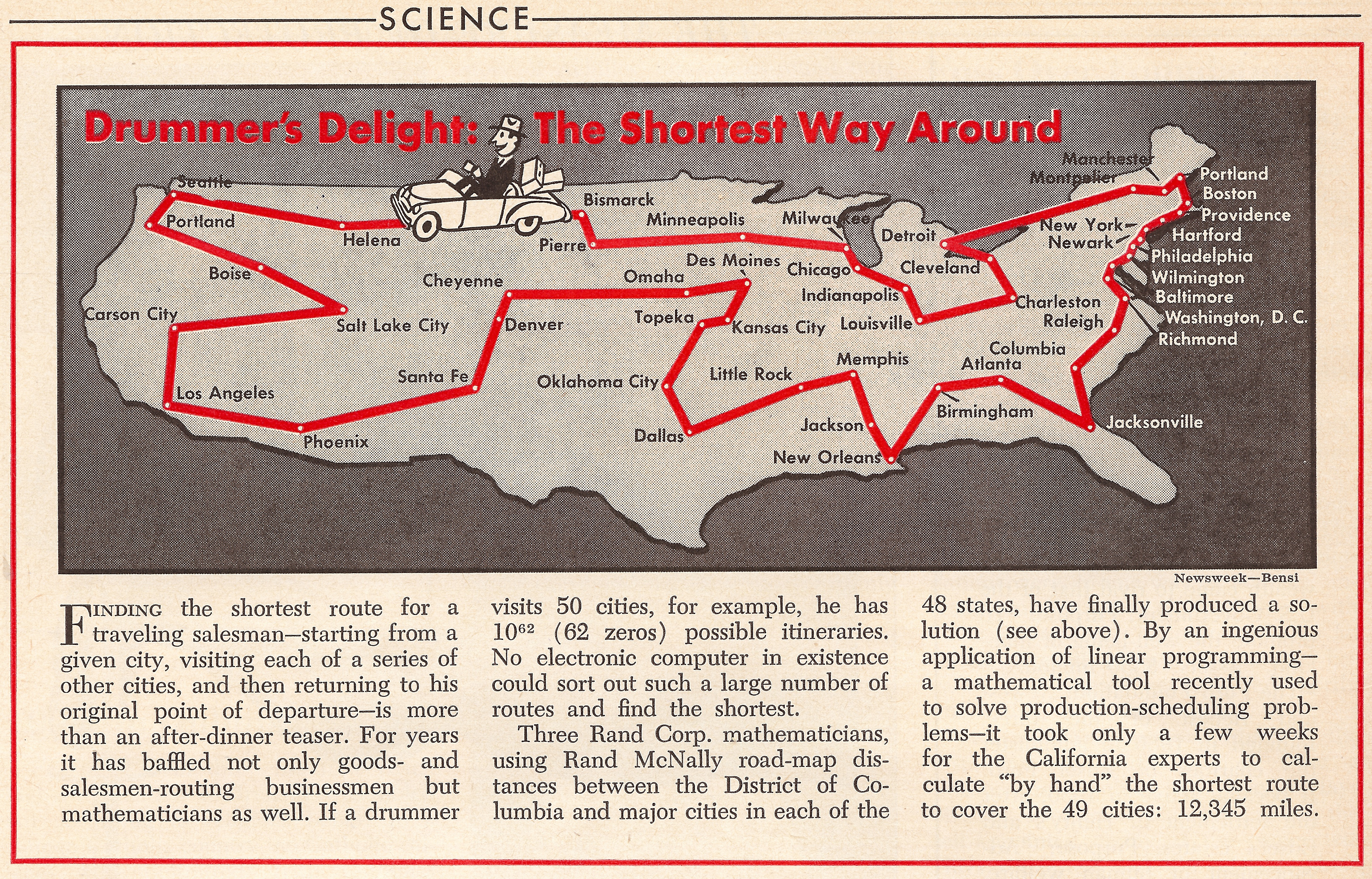
| Newsweek, July 26, 1954 |

March 2015 saw fantastic coverage of the traveling salesman problem in the media. A 50-city example, created by Tracy Staedter and Randy Olson, became a sensation, with articles in the Washington Post, NY Daily News, Daily Mail, People Magazine, NY Times, NPR, and many other outlets. Sometimes with Likes or Shares numbering in the 10,000s.
This is big news in itself, but it is not the first time a TSP tour of the USA has received attention. Back in 1954, Newsweek covered a mathematical sensation: three researchers at the Rand Corporation had solved the long-standing challenge of finding a shortest-possible route around cities in each of the 48 states plus Washington, D.C.
|
|
| Newsweek, July 26, 1954 |
The stunning feature of this 1954 work was that the researchers constructed a precise mathematical argument that their tour was shortest possible. That is, using the driving distance information they had in hand (taken from a Rand McNally atlas), they knew for certain that no route through the points was better than the one they had constructed. They proved they had an optimal tour.
Their technical paper appeared in the journal Operations Research with a beautifully succinct abstract.

|
This was brilliant work by George Dantzig, Ray Fulkerson, and Selmer Johnson. And we should all give them a great round of applause. The technique they crafted to attack the problem continues today to be a focal point of the research and practice of the applied mathematics and engineering fields called operations research and mathematical optimization.
The Newsweek article mentions that Dantzig's team harnessed the tool of linear programming (LP) to create a new solution method. Their technique now goes by the name branch-and-cut, and it applies much more generally than to the TSP alone. Earlier this year, Martin Groetschel, Lex Schrijver, and I commented on the importance of this optimization methodology, that grew out of the 1954 TSP work.
| In fact, today the LP-based branch-and-cut procedure is the corner stone of almost all commercial optimization software packages, and there is almost no product or service in the world where this methodology has not contributed to its design, manufacturing, or delivery. |
So cheers to Dantzig, Fulkerson and Johnson!
Fast forward to March 2015. The center of so much attention was a tour that visits Staedter's 50 locations and returns to the starting point. It was created by Randy Olson, who recently made a really cool post on a path-based method to find Waldo. In his 50-landmarks work, Olson employed one of the many available techniques for finding good-quality tours. His result is a good tour; about the quality one can obtain using a pencil and paper to trace out carefully a route by hand. (If you want to try for yourself, here is the point set without the tour; also as a pdf file.)

|
| Randy Olson Tour, March 2015 |
A misleading point in the current articles, however, is a claim that finding the absolute best possible tour is out of the question for modern computers. This claim is, of course, at odds with the 1954 Newsweek story. (Although, to be fair, Dantzig's team actually did all of their work with by-hand calculations; electronic computers were not plentiful back then.)
The impossibility claim is based on the observation that the number of tours grows extremely fast as the number of cities grows, and thus no computer in the world could examine all tours through the 50 locations.
This observation is correct: there are indeed a ton of tours through 50 points. But what is wrong is the assumption that to find the best possible route, we have to examine them all, one by one. Think about a similar problem of ordering a group of 50 students from smallest to tallest. There are as many possible orderings of the students as there are tours through the 50 points. Nonetheless, the students can get ordered in a snap. Well, maybe not a snap, but fairly quickly by comparing themselves to one another.
No one knows how to solve the TSP as quickly as sorting heights, but the mathematics of the TSP gives solution techniques much better than examining each and every tour. Dantzig, Fulkerson and Johnson told us how to do this, and it has been successfully employed on problems having many thousands of points. Here, for example, is a drawing of the shortest tour (traveling via helicopter, not driving) through all 13,509 cities in the continental USA that had a population of at least 500 people, at the time when it was solved in 1998.

|
| 13,509-city USA tour; Spektrum der Wissenschaft, April 1999 |
Solving a 13,509-city TSP takes some high-powered computing, but for Staedter's 50 landmarks, if we are given the travel distance between each pair of locations, we can find the absolute shortest tour through the full collection in a fraction of a second on a MacBook, or even an iPhone. And not only do we find the tour, we also know it is the best possible. (I should add that every student in my optimization course this semester turned in a TSP computer code for homework #2 in February, and all of their codes easily solve the 50-landmarks problem.)
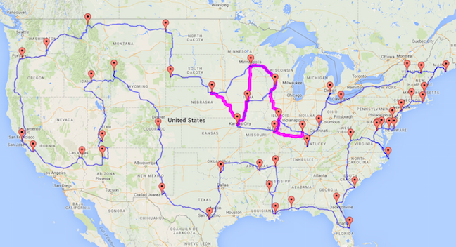
In contrast, the methodology adopted by Olson does not produce any guarantee on the quality of the tour it delivers. Nor is it competitive with any of the best non-guaranteed tour-finding methods that have been developed over the past 60 years. Indeed, the tour displayed in the many articles on the 50-landmarks problem is not the shortest possible, even when we use the same point-to-point distances provided by Google. It is not a bad tour, but it has a flaw in the order in which it visits locations in the center of the country. Here is an image that shows the mistake in the Olson tour.
|
|
The magenta path corrects the mistake in the Olson tour. |
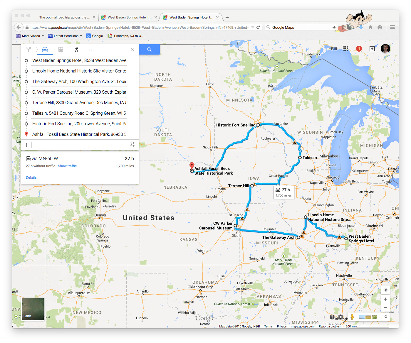
To convince you that this really is a mistake, here are two images I created with Google Maps, by typing in the wrong path (from the Olson tour) and the correct path (from the optimal tour). You can see that Google measures the wrong path as 1700 miles and the correct path as 1677 miles.
|

|
|
|
Wrong path: 1700 miles Click for larger version |
|
Correct path: 1677 miles Click for larger version |
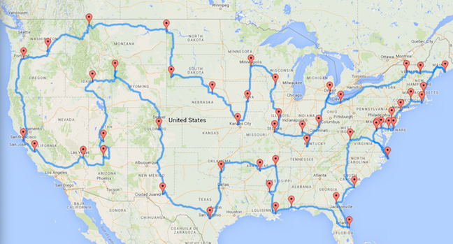
Below I show the optimal tour for the problem, assuming we adopt the travel distances (for driving) obtained from Google Maps with the same calls used by Randy Olson, to be able to compare apples with apples. Optimal means it is the shortest-possible route, measured in meters, using the prescribed point-to-point results from Google. (Note: We don't actually recommend this as a tour for visiting the 50 locations. Our recommended tour, taking in consideration the selection of point-to-point routing, is given on the On the Road page.)
|
|
The optimal tour for the 50-point TSP (with travel distances from Google via Randy Olson). |
It was easy to convince you that Olson's tour is not the best, but why should you believe the new tour is indeed the shortest possible (using the Google-Olson travel distances)? That is not so easy. What I'd like is to get you to read In Pursuit of the Traveling Salesman to see the mathematics that can convince you; the first chapter is available for free.
|
|
Failing that, here is what I can do: I offer a $10,000 reward to the first person who can find a better solution using our point-to-point distances. I don't recommend trying this, since there isn't a shorter tour, but if you want to give it a go, here is the table of travel distances (obtained from Google, as I described above) for each pair of cities. Each entry gives the travel distance in meters; the entries are ordered according to Staedter's list of the locations.
The length of the optimal tour is 22015038 meters. Just shave off a meter to win $10,000 (but be sure to use the table of distances to compute the length of your tour; the challenge is about getting a better ordering of the cities, not about finding a better point-to-point path to go from one city to another). For comparison, the length of Olson's tour is 22050978; so his result is 1.0016 times longer than the best tour.
To sum up, I'd say the idea of Tracy Staedter to tour USA landmarks was great, and Randy Olson's tour gives readers a nice chance to comment on the merits of visiting site X while site Y is just a bit further down the road. But if we want to talk about data geniuses, we better look to Dantzig, Fulkerson, and Johnson. Their work on the TSP changed the world!
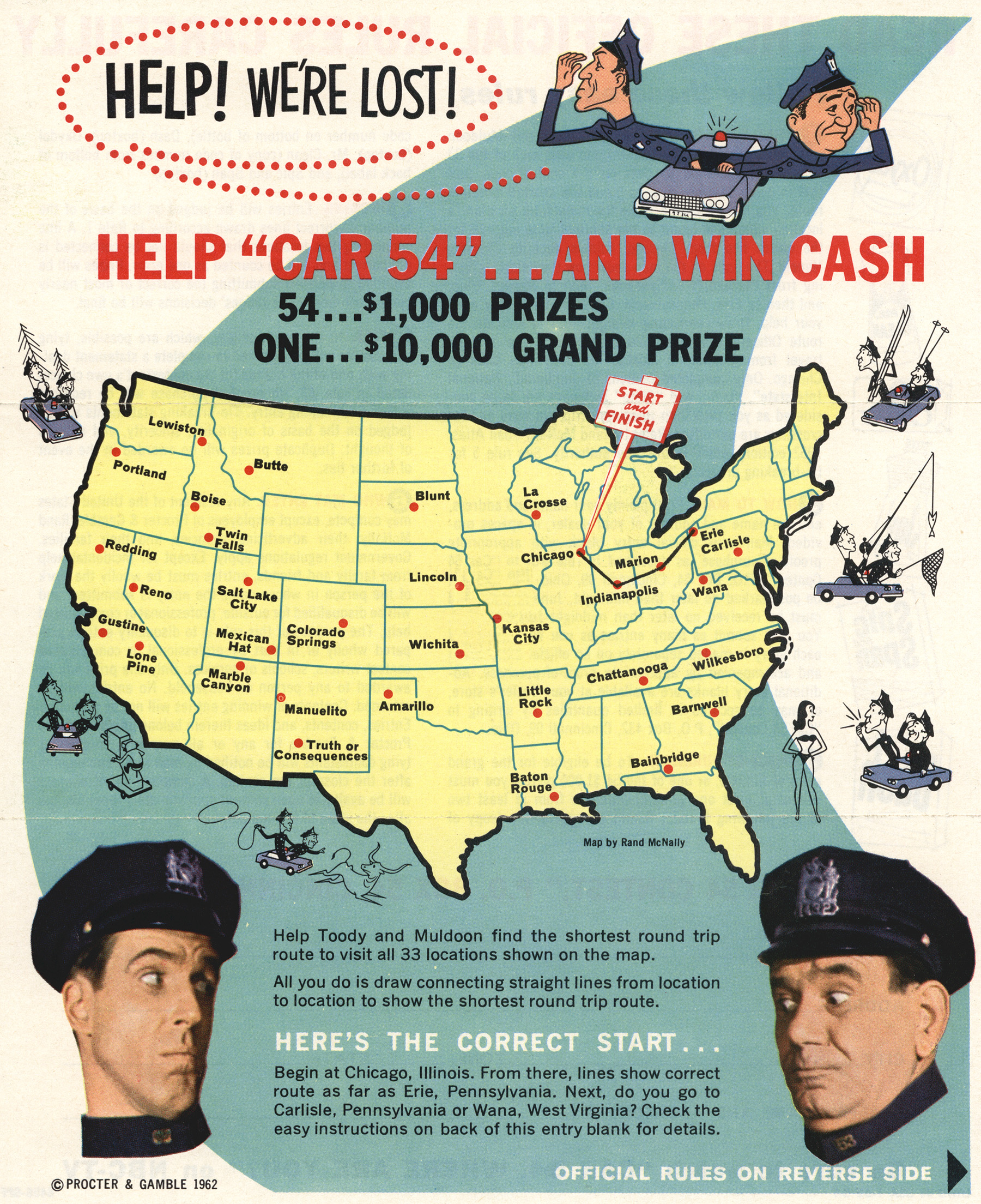
By the way, if you are desperate to earn $10,000 with a TSP tour, I should mention that Procter & Gamble ran a contest with that amount as the grand prize. The challenge was to find a short route through 33 cities, with distances taken from a Rand McNally atlas.
|
|
$10,000 TSP Contest from 1962. |
In this case, you need to also solve the time-travel problem, since the contest ran in 1962. The winning solutions were later shown to actually be optimal solutions (although the contestants did not know this at the time). So, even in 1962, good was not good enough.
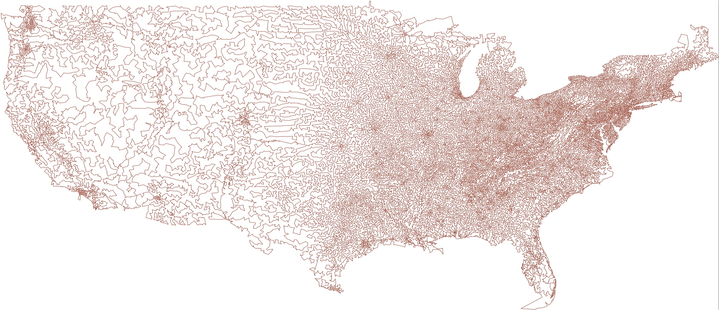
If money is not really your thing, then you are always welcome instead to join in and help with active computational research into the TSP. A current target is to find a proof that the tour pictured below is in fact an optimal tour through 115,475 towns and cities in the USA. You can read more about this TSP challenge here. We currently know, via the Dantzig-Fulkerson-Johnson techniques, that the tour is no more than 1.000096 times longer than an optimal tour. Shaving off that last 1/100th of a percent is going to take some new mathematics. And hopefully push further the limits of computatability, not just for the TSP, but for broad classes of optimization problems arising in society!
|
|
Is this the optimal tour through 115,475 towns and cities in the USA? |
![]()
Links to related pages
![]()
Randy Olson followed up his USA work by computing a tour through Europe. Here is the correction to his European tour.
![]()
Solving the USA road trip problem takes well under a second on my iPhone6. Thus, to see some action, I slowed the code down by adding sleep(1) commands and outputting extra graphics. You can watch the progress of the algorithm by running the QuickTime movie below. What you see is a fractional tour converging to an actual tour, which is provably the optimal solution.
![]()
The Lin-Kernighan hill-climbing heuristic starts with a random tour and repeatedly looks for possible improvements, removing sets of edges (colored red in the movie) and reconnecting the paths into a tour (using blue edges in the movie). In this example it finds the shortest-possible tour, but, unlike the linear-programming method used in Concorde, the algorithm does not know the tour is actually the optimal; it only knows that it does not see a way to improve it any further.
![]()
Note: This is not our recommended tour. For that, see the On the Road page.
Here is the list of sites in the order giving the optimal TSP tour (with the Google distances found by Randy Olson). Clicking on each link will take you to LatLong.net, where you can click on the Satellite box in the upper right to get a nice view of each landmark site. For GPS fans, I've also included an approximate latitude+longitude for each of the locations.